Unlocking Polymer Structure: The Mark-Houwink Equation in Biomedical Research and Drug Development
This comprehensive guide explores the Mark-Houwink equation, a fundamental relationship in polymer science linking intrinsic viscosity to molecular weight.
Unlocking Polymer Structure: The Mark-Houwink Equation in Biomedical Research and Drug Development
Abstract
This comprehensive guide explores the Mark-Houwink equation, a fundamental relationship in polymer science linking intrinsic viscosity to molecular weight. Designed for researchers and drug development professionals, it covers the theoretical foundations of the 'a' and 'K' parameters, practical methodologies for their determination using SEC, DLS, and viscometry, and strategies for troubleshooting experimental challenges. The article provides a comparative analysis of parameter sources and validation techniques, emphasizing critical applications in characterizing biopolymers, polymeric drug carriers, and hydrogel systems for clinical translation.
The Mark-Houwink Equation Explained: Core Principles and Parameter Significance
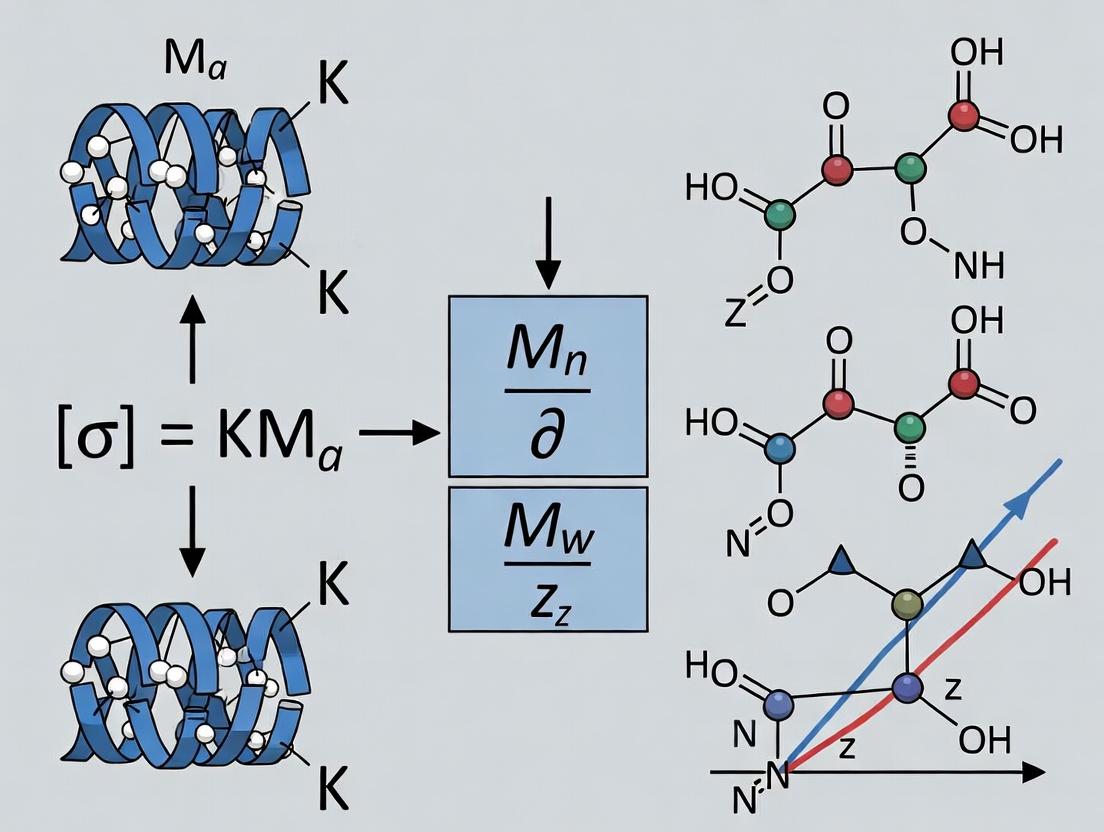
The Mark-Houwink-Sakurada equation, [η] = K M^a, is a cornerstone of polymer solution characterization. It relates the intrinsic viscosity [η] (mL/g) of a polymer in a specific solvent at a given temperature to its molecular weight (M). The parameters K and a are empirical constants that depend on the polymer-solvent-temperature system. Intrinsic viscosity reflects the hydrodynamic volume of a polymer coil in solution. The exponent a provides critical insight into the polymer's conformation: a value of 0.5-0.8 indicates a random coil in a theta or good solvent, 0.8-1.0 suggests a stiff rod-like chain, and ~0.5 denotes a compact sphere.
Application Notes: Data Compilation and Analysis
Recent research (2020-2024) continues to refine Mark-Houwink parameters for both established and novel polymers, particularly in biopharmaceutical contexts. The following table summarizes contemporary parameters for key therapeutic and research polymers.
Table 1: Contemporary Mark-Houwink Parameters for Selected Polymers (2020-2024)
| Polymer | Solvent | Temperature (°C) | K (mL/g) × 10^3 | a | Molecular Weight Range (Da) | Key Application/Note |
|---|---|---|---|---|---|---|
| Dextran | 0.1M NaNO₃ | 25 | 11.3 | 0.50 | 10⁴ – 10⁶ | Size-exclusion calibration standard. |
| Pullulan | 0.1M NaNO₃ | 25 | 16.6 | 0.65 | 10⁴ – 10⁶ | Biocompatible drug delivery, SEC standard. |
| Poly(L-lactic acid) (PLLA) | Chloroform | 25 | 21.5 | 0.77 | 10⁴ – 10⁶ | Biodegradable implants & microparticles. |
| Chitosan | 0.3M AcOH / 0.2M NaCl | 25 | 74.6 | 0.76 | 10⁴ – 10⁶ | Mucoadhesive drug delivery systems. |
| Monoclonal Antibody (IgG1) | PBS, pH 6.5 | 25 | 5.20 | 0.43 | ~1.5×10⁵ | Confirms near-globular native state in formulation. |
| Hyaluronic Acid | 0.15M NaCl | 25 | 22.8 | 0.79 | 10⁵ – 10⁷ | High a indicates stiff, expanded chain. |
| LNP-mRNA | Tris-EDTA Buffer | 25 | - | 0.10-0.30 | >1×10⁶ | Ultra-low a indicates highly compact, lipid-encapsulated structure. |
Key Insight: The data for monoclonal antibodies and lipid nanoparticles (LNPs) highlight the equation's utility beyond traditional synthetic polymers. The low a exponent for IgG1 (~0.43) confirms its compact, globular tertiary structure. The exceptionally low a for LNP-mRNA complexes quantitatively evidences their dense, particulate nature, crucial for stability and biodistribution profiling.
Experimental Protocols
Protocol 1: Determination of Intrinsic Viscosity ([η]) via Capillary Viscometry
Objective: To measure the intrinsic viscosity of a polymer sample as a prerequisite for Mark-Houwink analysis.
Materials:
- Ubbelohde-type capillary viscometer (suspended-level)
- Constant temperature bath (±0.01°C)
- Precision timer (±0.01 s)
- Polymer solutions at 4-5 concentrations (e.g., 0.2, 0.4, 0.6, 0.8 g/dL)
- Solvent (filtered, 0.2 µm)
Procedure:
- Clean and dry the viscometer. Mount it vertically in the temperature bath.
- Pipette ~15 mL of pure solvent into the viscometer. Allow 15 minutes for thermal equilibration.
- Measure the efflux time (t₀) at least five times; standard deviation should be <0.2%.
- Repeat step 3 for each polymer solution in order of increasing concentration.
- Calculate relative viscosity (ηrel = t / t₀), specific viscosity (ηsp = ηrel - 1), and reduced viscosity (ηred = η_sp / c).
- Plot both ηsp/c vs. c (Huggins plot) and (ln ηrel)/c vs. c (Kraemer plot).
- Extrapolate both plots to zero concentration (c→0). The common y-intercept is the intrinsic viscosity [η] (in mL/g).
Protocol 2: Establishing Mark-Houwink Parameters via SEC-MALS-Viscosity
Objective: To determine K and a for a new polymer-solvent system using absolute molecular weight detection.
Materials:
- Size-Exclusion Chromatography (SEC) system with isocratic pump and autosampler.
- Multi-Angle Light Scattering (MALS) detector.
- Differential viscometer (DV) detector.
- Refractive Index (RI) detector.
- Appropriate SEC columns (matched to polymer size range).
- Known narrow dispersity polymer standards for system calibration (optional for MALS absolute method).
- Polymer samples with broad molecular weight distribution.
Procedure:
- System Setup: Connect detectors in series: SEC → MALS → DV → RI. Equilibrate with filtered, degassed solvent at fixed flow rate (e.g., 1.0 mL/min).
- Calibration: Inject a narrow standard (e.g., polystyrene) to verify inter-detector delay volumes and band broadening. Align data from all detectors.
- Sample Analysis: Inject individual polymer samples of known, broad molecular weight distribution. For each slice i of the chromatogram, the system simultaneously measures:
- Mi: Absolute molecular weight from MALS (and RI concentration).
- [η]i: Intrinsic viscosity from the differential viscometer.
- Data Processing: Collect paired data points (Mi, [η]i) across the entire chromatogram peak.
- Parameter Calculation: Perform a linear least-squares regression on the log-transformed data: log([η]i) = log(K) + a * log(Mi). The slope yields exponent a, and the antilog of the intercept yields constant K.
- Validation: Verify parameters using a second, independent set of polymer samples or literature values.
Visualizations
Title: Physical Meaning of Mark-Houwink Parameters
Title: SEC-MALS-Viscometry Workflow for K & a
The Scientist's Toolkit: Essential Research Reagents & Materials
Table 2: Key Reagents and Materials for Mark-Houwink Studies
| Item | Function/Brief Explanation |
|---|---|
| Ubbelohde Capillary Viscometer | Glass viscometer designed for precise kinematic viscosity measurements; minimizes errors from head pressure. |
| Multi-Angle Light Scattering (MALS) Detector | Provides absolute molecular weight for each eluting fraction without reliance on column calibration standards. |
| Differential Viscometer (DV) Detector | Measures specific viscosity directly by comparing pressure drops across capillaries for solution and solvent. |
| Narrow Dispersity Polymer Standards | (e.g., Polystyrene, PEG, Dextran) Used for SEC column calibration and system verification. |
| 0.2 µm PTFE Membrane Filters | For critical filtration of all solvents and solutions to remove dust and particulate matter, essential for light scattering. |
| Precision Temperature Bath (±0.01°C) | Temperature control is critical as viscosity and polymer conformation are highly temperature-dependent. |
| Refractive Index (RI) Detector | Measures polymer concentration in SEC eluent, required for both [η] and Mw calculation with MALS. |
| Appropriate SEC Columns | (e.g., TSKgel, PLgel) Matched pore sizes to the polymer's hydrodynamic radius range for optimal separation. |
| High-Purity, Anhydrous Solvents | Solvent purity directly impacts polymer-solvent interactions and the accuracy of K and a parameters. |
| Data Acquisition/Analysis Software | Specialized software (e.g., Astra, OMNISEC) is required to synchronize and analyze multi-detector SEC data. |
Within the framework of polymer solutions research, the Mark-Houwink-Sakurada (MHS) equation, [η] = K Mˣ, is a cornerstone for correlating intrinsic viscosity [η] with molecular weight (M). The parameters 'a' and 'K' are not mere fitting constants; they are profound indicators of polymer conformation and solvent-polymer interaction. This application note details the contemporary interpretation, determination, and application of these parameters, providing protocols for their experimental derivation and analysis, crucial for researchers in biomaterials and drug delivery system development.
Theoretical Foundation & Contemporary Interpretation
The exponent 'a' reflects the hydrodynamic volume and chain conformation of a polymer in a specific solvent. The constant 'K' is influenced by polymer stiffness, solvent quality, and temperature. Current research emphasizes their role in predicting nanoparticle hydrodynamic size in solution, critical for drug delivery vector design.
Table 1: Theoretical Ranges and Conformational Significance of the MHS Exponent 'a'
| 'a' Value Range | Polymer Conformation | Solvent Quality | Typical Polymer Examples |
|---|---|---|---|
| 0.5 - 0.6 | Compact sphere, poor solvent conditions | Poor (Theta solvent) | Dense globular proteins |
| ~0.7 | Flexible coil in theta conditions | Theta (θ) | Polystyrene in cyclohexane at 34.5°C |
| 0.7 - 0.9 | Flexible random coil | Good | Poly(methyl methacrylate) in acetone |
| >0.9 (up to ~1.8) | Rigid rod, stiff chain, or elongated coil | Good to excellent | Cellulose derivatives, chitosan in specific solvents, DNA |
Table 2: Factors Influencing the MHS Constant 'K'
| Factor | Effect on 'K' | Molecular Implication |
|---|---|---|
| Polymer Chain Stiffness | Increases | Higher hydrodynamic volume per unit mass. |
| Solvent Quality Improvement | Increases | Chain expansion increases effective volume. |
| Increase in Temperature | Variable | Depends on solvent-polymer interaction enthalpy. |
| Branching (vs. Linear) | Decreases | More compact molecular architecture. |
Experimental Protocol: Determining 'a' and 'K' for a Novel Polymer
This protocol outlines the steps to establish a Mark-Houwink relationship for an unknown polymer sample.
A. Materials & Reagent Solutions
Table 3: Research Reagent Solutions & Essential Materials
| Item / Reagent | Function / Explanation |
|---|---|
| Polymer Samples | Narrow molecular weight distribution (Ð < 1.1) standards of the polymer of interest (at least 5 standards). |
| Appropriate Solvent | High-purity solvent, thoroughly degassed to prevent bubble formation in viscometers. |
| Ubbelohde Capillary Viscometer | Glass viscometer for measuring efflux times; enables dilution series without changing total volume. |
| Multi-Angle Light Scattering (MALS) Detector | Coupled with SEC for absolute molecular weight determination of standards/unknowns. |
| Size Exclusion Chromatography (SEC) System | For separating polymer by hydrodynamic size and analyzing polydispersity. |
| Temperature-Controlled Bath | Maintains viscometry measurements at constant temperature (±0.1°C). |
| Precision Timer | For accurate efflux time measurement. |
| Differential Refractometer (dRI) / UV Detector | For concentration detection in SEC. |
B. Step-by-Step Methodology
Part I: Intrinsic Viscosity ([η]) Measurement via Dilution Viscometry
- Solution Preparation: Prepare stock solutions of each polymer standard at a known, precise concentration (c₀, typically 0.5-1.0 g/dL). Filter through a 0.2 μm membrane filter.
- Viscometer Calibration: Clean and dry the Ubbelohde viscometer. Load the pure, degassed solvent and equilibrate in the temperature bath (e.g., 25.0°C ± 0.1°C) for 15 minutes. Measure the efflux time (t₀) in triplicate. The average should have low variance (< 0.2%).
- Dilution Series: Load the polymer stock solution into the viscometer. Measure its efflux time (t). Sequentially dilute the solution within the viscometer by adding measured volumes of solvent, and measure efflux times at each concentration (c).
- Data Processing: Calculate the relative viscosity (ηrel = t/t₀), specific viscosity (ηsp = ηrel - 1), and reduced viscosity (ηred = ηsp / c). Plot both ηred and (ln η_rel)/c versus concentration (c).
- Determination of [η]: Perform a linear extrapolation of both plots to zero concentration (c → 0). The y-intercept from both plots should converge to the same value, which is the intrinsic viscosity [η]. Repeat for all polymer standards.
Part II: Absolute Molecular Weight Determination (for Standards)
- SEC-MALS Setup: Calibrate the SEC system with the appropriate solvent and flow rate. Ensure the MALS and dRI detectors are normalized and the inter-detector delay volume is calibrated.
- Analysis: Inject each narrow dispersity polymer standard. The MALS detector provides the absolute weight-average molecular weight (M_w) directly from the scattered light intensity without reliance on elution time standards.
- Validation: The reported Mw for each standard should match its certificate value within uncertainty. Record the Mw value for each standard.
Part III: Establishing the Mark-Houwink Relationship
- Data Pairing: You now have paired data: [η]ᵢ and M_wᵢ for each polymer standard 'i'.
- Log-Log Plot: Construct a plot of log₁₀[η] versus log₁₀ M_w.
- Linear Regression: Perform a least-squares linear regression on the data. The slope of the line is the Mark-Houwink exponent 'a'. The y-intercept (log₁₀[η] at log₁₀ Mw = 0, i.e., Mw = 1 g/mol) is log₁₀ K, from which K is calculated.
C. Data Analysis & Visualization
Title: Workflow for Determining Mark-Houwink Parameters
Application Protocol: Using MHS Parameters to Infer Conformation
Objective: Characterize the solution conformation of an unknown polymer batch or a polymer in a new solvent.
Procedure:
- Determine the intrinsic viscosity ([η]_unk) of your unknown sample using Protocol 2, Part I.
- Determine its absolute molecular weight (Mwunk) using SEC-MALS (Protocol 2, Part II).
- Using the established Mark-Houwink equation ([η] = K Mˣ) from your standards:
- Calculate the expected intrinsic viscosity: [η]exp = K * (Mw_unk)ˣ.
- Compare [η]exp with the measured [η]unk.
- Interpretation:
- If [η]unk ≈ [η]exp, the unknown polymer likely shares the same conformation as the standards in that solvent.
- If [η]unk < [η]exp, the unknown polymer is more compact (e.g., branched, aggregated, or in a poorer solvent).
- If [η]unk > [η]exp, the unknown polymer is more expanded (e.g., more rigid, charged, or in a better solvent).
- Calculate the Conformation-Sensitive Exponent for the Unknown: Using the measured pair ([η]unk, Mwunk), calculate asingle = (log[η]unk - log K) / log Mw_unk. Compare this single-point 'a' value to the theoretical ranges in Table 1.
Title: Logic for Conformational Analysis Using MHS Parameters
Advanced Considerations & Data Tables
For drug development, understanding batch-to-batch consistency or conjugation effects is vital.
Table 4: Impact of Common Polymer Modifications on MHS Parameters
| Polymer Modification | Expected Impact on 'a' | Expected Impact on 'K' | Rationale |
|---|---|---|---|
| PEGylation | Decrease (slight) | Variable | Shielding and possible crowding can lead to a more compact hydrodynamic sphere. |
| Introduction of Charged Groups | Increase | Increase | Electrostatic repulsion expands the chain (polyelectrolyte effect). |
| Controlled Branching | Decrease | Decrease | Branched polymers are more compact than their linear counterparts of equal M_w. |
| Hydrolysis (e.g., of PLA) | Increase | Increase | Chain scission reduces M_w, but new chain ends may increase polarity/solvation. |
Table 5: Example MHS Parameters for Biopolymers (Recent Literature)
| Polymer | Solvent | Temp (°C) | K (mL/g) | a | Conformational Inference |
|---|---|---|---|---|---|
| Dextran (linear) | Water / 0.1M NaNO₃ | 25 | 0.023 | 0.65 | Flexible coil near theta conditions. |
| Chitosan (medium DA) | 0.3M Acetic acid / 0.2M NaCl | 25 | 0.074 | 0.76 | Flexible chain in good solvent. |
| Hyaluronic Acid | 0.1M NaCl (PBS) | 25 | 0.029 | 0.78 | Semi-flexible polyelectrolyte in screened conditions. |
| PLGA (50:50) | Tetrahydrofuran (THF) | 30 | 0.056 | 0.67 | Flexible coil. |
Within the broader thesis on determining Mark-Houwink parameters for polymer solutions, establishing the theoretical foundation linking polymer chain dimensions to hydrodynamic volume is paramount. The Mark-Houwink equation, [η] = K M^a, intrinsically connects the intrinsic viscosity [η] (a hydrodynamic property) to the polymer molar mass M. The exponent a is a direct reflection of the polymer-solvent thermodynamic interaction and the resulting chain dimensions in solution. This application note details the experimental protocols and theoretical models used to quantify chain dimensions (e.g., radius of gyration, Rg; hydrodynamic radius, Rh) and their relationship to the parameters K and a.
Theoretical Framework: Key Models and Quantitative Data
The value of the Mark-Houwink exponent a is interpreted through polymer chain models.
Table 1: Theoretical Mark-Houwink Exponents & Chain Dimensions
| Polymer Chain Model & Solvent Condition | Theta (θ) Temperature? | Chain Dimension Scaling (Rg ∝ M^ν) | Theoretical Mark-Houwink Exponent a |
Expected a Range (Experimental) |
|---|---|---|---|---|
| Hard-Sphere (Impenetrable) | N/A | N/A | 0 | ~0 |
| Free-Draining Chain (No Hydrodynamic Interaction) | Any | Rg ∝ M^0.5 | 0.5 | Rarely observed |
| Non-Free-Draining, Theta Solvent (θ-condition) | Yes | Rg ∝ M^0.5 | 0.5 | 0.5 |
| Non-Free-Draining, Good Solvent | No | Rg ∝ M^0.588 (Flory) | 0.588 (Flory) | 0.6 - 0.8 |
| Rigid Rod | N/A | Rg ∝ M^1 | 1.8 | ~1.8 |
| Semi-Flexible Chain / Wormlike Chain | Dependent on Persistence Length | Variable | 0.5 - 1.8 | Dependent on stiffness |
Table 2: Key Universal Ratios for Polymer Characterization
| Universal Ratio | Definition | Theoretical Value (θ-solvent) | Theoretical Value (Good Solvent) | Experimental Method for Determination |
|---|---|---|---|---|
| ρ-parameter (Shape Factor) | ρ = Rg / Rh | ~1.5 | ~1.8 - 2.0 | Combined SEC-MALS-DLS |
| Flory Constant (Φ) | Φ = [η]M / (Rg^3) | ~2.6 × 10^23 mol^-1 | ~2.5 × 10^23 mol^-1 | Viscometry + SEC-MALS |
| Viscosity-Radius Ratio | [η]M / (Rh^3) | - | - | Viscometry + SEC-DLS |
Experimental Protocols
Protocol 3.1: Determining Chain Dimensions via Multi-Angle Light Scattering (MALS) with Size-Exclusion Chromatography (SEC)
Objective: To measure the absolute molar mass (Mw) and the root-mean-square radius of gyration (Rg) across a polymer fractionation.
Materials & Reagents:
- SEC system with isocratic pump, autosampler, and column oven.
- MALS detector (e.g., Wyatt DAWN, Brookhaven BI-MwA).
- Differential Refractometer (dRI) for concentration detection.
- Appropriate SEC columns (e.g., Agilent PLgel, Tosoh TSKgel).
- High-quality solvent (HPLC grade, e.g., THF, DMF, aqueous buffer), filtered through 0.1 µm filter.
- Polymer standards for system calibration/validation (e.g., narrow dispersity polystyrene).
Procedure:
- System Preparation: Dissolve polymer sample in the mobile phase at a known concentration (typically 1-5 mg/mL). Filter through a 0.22 or 0.45 µm syringe filter (PTFE for organic, nylon for aqueous).
- SEC-MALS Setup: Equilibrate the SEC columns with mobile phase at a constant flow rate (e.g., 1.0 mL/min for analytical columns). Ensure MALS and dRI detectors are stabilized.
- Data Collection: Inject an appropriate volume (50-100 µL). The SEC system fractionates the polymer by hydrodynamic size. Each eluting slice is analyzed by MALS (measuring scattered light intensity at multiple angles) and dRI (measuring concentration).
- Data Analysis: Use specialized software (e.g., ASTRA, Zimm fit) to analyze the angular dependence of scattered light for each slice. The Zimm equation is applied:
(K*c)/R(θ) = 1/Mw * (1 + (16π²n₀²/3λ₀²) * Rg² * sin²(θ/2)) + 2A₂c. From the slope ofK*c/R(θ)vs.sin²(θ/2), Rg is calculated. The intercept yields Mw. - Validation: Run a monodisperse standard (e.g., BSA for aqueous) to verify system alignment and accuracy.
Protocol 3.2: Determining Hydrodynamic Radius via Dynamic Light Scattering (DLS)
Objective: To measure the hydrodynamic radius (Rh) of a polymer in solution via analysis of intensity fluctuation of scattered light.
Materials & Reagents:
- DLS instrument (e.g., Malvern Zetasizer, Wyatt DynaPro).
- Disposable or quartz cuvettes (low volume, ~12 µL to 1 mL).
- Solvent (filtered through 0.02 µm filter).
- Polymer sample.
Procedure:
- Sample Preparation: Prepare polymer solutions at multiple concentrations (e.g., 0.1, 0.5, 1.0 mg/mL) in filtered solvent. Clarify by centrifugation or filtration if necessary.
- Measurement: Load the sample into a clean cuvette, place in the thermostatted sample chamber. Set the instrument parameters (temperature, equilibration time, laser wavelength, scattering angle).
- Data Acquisition: Run the measurement to collect the intensity autocorrelation function,
g²(τ). - Data Analysis: The software fits
g²(τ)to derive the diffusion coefficientDusing the Cumulants method or CONTIN algorithm. The hydrodynamic radiusRhis calculated via the Stokes-Einstein equation:Rh = kT / (6πηD), wherekis Boltzmann's constant,Tis temperature, andηis solvent viscosity. - Concentration Series: Perform measurements across concentrations and extrapolate
Rhto zero concentration to obtain the value free of intermolecular interactions.
Protocol 3.3: Determining Intrinsic Viscosity via Capillary Viscometry
Objective: To measure the intrinsic viscosity [η] of a polymer solution, the key parameter for the Mark-Houwink equation.
Materials & Reagents:
- Glass capillary viscometer (e.g., Ubbelohde type, Cannon).
- Constant temperature bath (±0.01°C).
- Digital stopwatch.
- High-precision polymer solutions at 4-5 different concentrations.
Procedure:
- Solvent Flow Time: Clean and dry the viscometer. Fill with filtered solvent. Immerse in the constant temperature bath (typically 25°C or 30°C). Allow thermal equilibration (15 min). Measure the efflux time
t₀at least five times; standard deviation should be <0.2 seconds. - Solution Flow Times: Prepare polymer solutions of known concentrations
c(e.g., 0.2, 0.4, 0.6, 0.8 g/dL). For each, fill the viscometer, equilibrate, and measure the efflux timet. - Data Processing: Calculate the relative viscosity
η_rel = t/t₀. Calculate specific viscosityη_sp = η_rel - 1. - Determination of [η]: Plot both
(η_sp / c)and(ln(η_rel) / c)versus concentrationc. Extrapolate both plots to zero concentration. The common intercept is the intrinsic viscosity[η]. - Mark-Houwink Plot: For a series of fractionated polymer samples with known
M(from SEC-MALS), plotlog([η])vs.log(M). Perform a linear fit; the slope isaand the intercept islog(K).
Visualizations
Diagram 1: Polymer Hydrodynamics to Mark-Houwink Parameters
Diagram 2: Experimental Workflow for Parameter Determination
The Scientist's Toolkit: Research Reagent Solutions
Table 3: Essential Materials for Polymer Hydrodynamics Research
| Item / Reagent Solution | Function & Purpose | Key Considerations for Selection |
|---|---|---|
| SEC-MALS-dRI System | Integrated system for absolute molar mass, size, and concentration measurement. | Choose detectors compatible with your solvent (aqueous/organic). MALS detector with ≥18 angles provides superior Rg data. |
| DLS Instrument | Measures hydrodynamic radius (Rh) and polydispersity via diffusion coefficient. | Consider sample volume requirements, temperature range, and ability to measure at multiple angles. |
| Ubbelohde Viscometer | Measures intrinsic viscosity [η] via precise flow time measurements. |
Select capillary size (e.g., 0B, 0C, 1) appropriate for expected [η] range. |
| Chromatography Columns | Separates polymer by hydrodynamic size (SEC mode). | Match pore size to polymer molar mass range (e.g., mixed-bed, linear). Ensure chemical compatibility with solvent. |
| Ultra-pure, Filtered Solvents | Mobile phase and sample solvent. Must be particle-free. | Use HPLC grade. Always filter through 0.1 µm filter for SEC, 0.02 µm for DLS. Degas for viscometry. |
| Narrow Dispersity Polymer Standards | Calibration/validation of SEC-MALS-DLS system and theory. | Polystyrene (THF), PEG/PEO (aqueous), Pullulan (aqueous). Certified Mw and Đ values are essential. |
| Syringe Filters (PTFE, Nylon) | Removes dust and aggregates prior to injection, critical for light scattering. | 0.22 µm or 0.45 µm pore size. PTFE for organic solvents, nylon or PVDF for aqueous buffers. |
| Specialized Software (ASTRA, Zetasizer) | Data acquisition and analysis for light scattering, SEC, and viscometry. | Required for fitting Zimm plots, calculating Rh from correlation functions, and Mark-Houwink analysis. |
The Mark-Houwink equation, [η] = K Mˣ, relates the intrinsic viscosity [η] of a polymer solution to its molar mass (M). The parameters 'a' (the Mark-Houwink exponent) and 'K' are not universal constants but are profoundly influenced by the polymer-solvent system and conditions. Within the broader thesis on polymer solutions research, this application note details the experimental determination and analysis of how solvent quality, temperature, and polymer architecture affect 'a' and 'K', which are critical for accurate molar mass characterization in fields like pharmaceuticals and material science.
Influence of Solvent Quality
Solvent quality dictates polymer chain conformation, directly impacting intrinsic viscosity.
Table 1: Typical Mark-Houwink Parameters for Polystyrene in Different Solvents at 25°C
| Solvent | Quality | 'a' value | Log₁₀ K (dL/g) | Chain Conformation |
|---|---|---|---|---|
| Cyclohexane (θ-cond., 34.5°C) | Theta | 0.50 | -4.22 | Unperturbed coil |
| Toluene | Good | 0.73 | -3.87 | Expanded coil |
| Dichloromethane | Very Good | 0.79 | -3.99 | Highly expanded coil |
Protocol: Determining 'a' and 'K' for a New Solvent System
Objective: Establish Mark-Houwink parameters for a polymer in an unknown solvent. Materials: Polymer samples with narrow dispersity (Đ < 1.1) across a molar mass range (e.g., 5 standards, 10kDa to 500kDa), target solvent, viscometer (e.g., Ubbelohde), SEC-MALS system. Procedure:
- Sample Preparation: Precisely dissolve each polymer standard in the solvent at known concentrations (typically 0.5-2 mg/mL). Filter solutions (0.45 µm PTFE filter).
- Intrinsic Viscosity Measurement:
- Use an automated viscometer or perform manual flow time measurements in an Ubbelohde viscometer at constant temperature (±0.1°C).
- For each standard, measure flow times (t) for at least 3 concentrations and the pure solvent (t₀).
- Calculate relative (ηᵣ = t/t₀), specific (ηₛₚ = ηᵣ - 1), and reduced viscosity (ηᵣₑd = ηₛₚ/c).
- Plot ηₛₚ/c vs. c and (ln ηᵣ)/c vs. c. Extrapolate both to infinite dilution (c→0) to obtain [η] as the common intercept.
- Molar Mass Confirmation: Analyze each standard via SEC coupled with Multi-Angle Light Scattering (MALS) and a refractive index (RI) detector in the same solvent to obtain absolute weight-average molar mass (Mʷ).
- Data Analysis: Plot log₁₀[η] vs. log₁₀ Mʷ for all standards. Perform linear regression. The slope is the exponent 'a', and the intercept is log₁₀ K.
Influence of Temperature
Temperature affects solvent quality and polymer chain dynamics.
Table 2: Effect of Temperature on 'a' for Poly(methyl methacrylate) in Various Solvents
| Polymer | Solvent | Temperature (°C) | 'a' value | Notes |
|---|---|---|---|---|
| PMMA | Acetone | 25 | 0.69 | - |
| PMMA | Acetone | 40 | 0.71 | Improved solvent quality |
| PMMA | Butanone | 25 | 0.72 | - |
| PMMA | Butanone | 50 | 0.74 | Improved solvent quality |
| PMMA | Isobutyraldehyde (θ-solvent) | 40 | 0.50 | Theta condition |
Protocol: Measuring Temperature Dependence of [η]
Objective: Assess the thermodynamic quality of a solvent by evaluating the temperature coefficient of intrinsic viscosity. Materials: Ubbelohde viscometer, precision temperature-controlled bath (±0.01°C), polymer solution. Procedure:
- Prepare a single polymer solution at a suitable concentration.
- Immerse the viscometer in the temperature bath, allowing equilibration for at least 15 minutes per set point.
- Measure flow times at a minimum of 5 temperatures spanning a range (e.g., 25°C to 50°C).
- Calculate [η] at each temperature using the Huggins plot method (as in Protocol 1.2).
- Plot [η] vs. Temperature. An increasing trend indicates an endothermic mixing process (common for good solvents). A distinct maximum or changing slope may indicate conformational transitions.
Influence of Polymer Architecture
Chain architecture (linear, branched, star, cyclic) fundamentally alters hydrodynamic volume.
Table 3: Mark-Houwink Parameters for Different Polymer Architectures (Example: Polystyrenes)
| Architecture | 'a' value (range) | Notes (vs. Linear Analog) |
|---|---|---|
| Linear | 0.70 - 0.76 | Reference |
| Comb / Branched | 0.30 - 0.65 | Lower 'a' and [η] due to compactness |
| Star (4-arm) | ~0.55 | More compact, lower 'a' |
| Ring / Cyclic | ~0.66 (at high M) | More compact than linear at same M |
Protocol: Distinguishing Architecture via Viscometry-SEC
Objective: Identify architectural deviations from linearity using universal calibration. Materials: SEC system with RI, viscometer (VISC), and light scattering (LS) detectors; linear narrow standards; unknown polymer sample. Procedure:
- Universal Calibration: Perform SEC analysis of linear polystyrene (or other polymer) standards. Plot log₁₀ ([η]·M) vs. elution volume (Vₑ) to construct a universal calibration curve.
- Sample Analysis: Inject the unknown architecture polymer under identical SEC conditions.
- Data Processing:
- From the VISC detector, obtain [η] at each slice.
- From the LS detector, obtain absolute M at each slice.
- Calculate the hydrodynamic volume ([η]·M) for each slice of the unknown.
- Architectural Plot: Plot log₁₀ ([η]·M) for the unknown against its Vₑ. Overlay the universal calibration line.
- If the unknown data falls on the line, it has a similar conformation to the linear standard.
- If it falls below the line, it has a more compact architecture (e.g., branched, star) for a given Vₑ (hydrodynamic size).
The Scientist's Toolkit: Research Reagent Solutions
Table 4: Essential Materials for Mark-Houwink Parameter Determination
| Item | Function |
|---|---|
| Narrow Dispersity Polymer Standards | Provide monodisperse samples for establishing precise log [η] vs. log M plots. |
| High-Purity, Anhydrous Solvents | Ensure consistent solvent quality and prevent aggregation or degradation. |
| Ubbelohde Capillary Viscometer | Measures relative flow time for intrinsic viscosity calculation via extrapolation. |
| Online Viscometer Detector (e.g., VISC) | Measures intrinsic viscosity at each SEC elution slice for universal calibration. |
| Multi-Angle Light Scattering (MALS) Detector | Provides absolute molar mass measurement independent of elution volume. |
| Refractive Index (RI) Detector | Measures polymer concentration in SEC for calculating [η] and concentration profiles. |
| PTFE Syringe Filters (0.1µm & 0.45µm) | Removes dust and aggregates to prevent scattering artifacts and column damage. |
Visualizations
Title: Solvent Quality Affects Mark-Houwink Parameters
Title: Protocol for Temperature Dependence of [η]
Title: SEC Workflow to Detect Polymer Architecture
Application Notes
Within the broader thesis on determining and applying Mark-Houwink equation parameters for polymer solutions research, viscometry serves as a foundational analytical technique. It provides a critical bridge between a simple, accessible measurement—viscosity—and the fundamental polymer property of molecular weight (MW). The Mark-Houwink-Sakurada equation, [η] = K * M^a, establishes this relationship, where [η] is the intrinsic viscosity, M is the molecular weight, and K and a are empirical constants specific to the polymer-solvent-temperature system.
For researchers, scientists, and drug development professionals, this bridge is indispensable. In biopharmaceuticals, the intrinsic viscosity of monoclonal antibodies or protein conjugates is a key indicator of solution behavior, aggregation propensity, and manufacturability. For synthetic polymers used in drug delivery (e.g., PLGA, PEG), it enables rapid batch-to-batch MW assessment without advanced instrumentation. Accurate K and a parameters are paramount; they transform viscometry from a qualitative test into a quantitative tool for molecular weight determination, conformational analysis (via the a exponent), and ultimately, predicting in-vivo performance and stability.
Table 1: Representative Mark-Houwink Parameters for Common Polymers in Pharmaceutical Research
| Polymer | Solvent | Temperature (°C) | K (dL/g) | a value | Molecular Weight Range (Da) | Conformation Indicated |
|---|---|---|---|---|---|---|
| Polystyrene (atactic) | Toluene | 25 | 1.10 x 10⁻⁴ | 0.725 | 50,000 - 2,000,000 | Random Coil (Good Solvent) |
| Poly(lactic-co-glycolic acid) (PLGA 50:50) | Tetrahydrofuran (THF) | 30 | 2.13 x 10⁻⁴ | 0.639 | 10,000 - 150,000 | Random Coil |
| Poly(ethylene glycol) (PEG) | Water | 25 | 6.86 x 10⁻⁴ | 0.500 | 2,000 - 40,000 | Theta Condition |
| Dextran | Water (0.1M NaCl) | 25 | 9.78 x 10⁻⁴ | 0.500 | 10,000 - 500,000 | Near-Theta Condition |
| Monoclonal Antibody (IgG1) | PBS, pH 6.5 | 25 | 2.37 x 10⁻⁵ | 0.71 | ~150,000 | Compact, Globular |
Table 2: Intrinsic Viscosity Determination Methods Comparison
| Method | Description | Typical Sample Volume | Key Advantage | Primary Limitation |
|---|---|---|---|---|
| Capillary (Ubbelohde) | Measures flow time of polymer solution vs. pure solvent. | 5-15 mL | High precision, absolute measurement. | Requires large, purified sample; multiple concentrations needed. |
| Micro-Viscometer | Miniaturized capillary system. | 100-500 µL | Low sample consumption. | Sensitive to bubbles and particulates. |
| Parallel Plate Rheometry | Measures viscosity under defined shear stress/rate. | 0.5-2 mL | Direct shear-thinning analysis. | Not ideal for dilute solutions; instrument complexity. |
| Size Exclusion Chromatography (SEC) with Viscosity Detection | Couples SEC separation with in-line viscometer. | 50-100 µL (injected) | Provides [η] across MW distribution. |
Requires SEC system and column calibration. |
Experimental Protocols
Protocol 1: Determination of Intrinsic Viscosity[η]using an Ubbelohde Viscometer
Objective: To obtain the intrinsic viscosity of a dilute polymer solution via serial dilution in a capillary viscometer and extrapolate to zero concentration.
Materials: See "The Scientist's Toolkit" below.
Procedure:
- Solvent Preparation & Viscometer Calibration: Dry and filter the solvent. Clean the Ubbelohde viscometer with chromic acid (or appropriate solvent) and dry thoroughly. Pipette a known volume (e.g., 12 mL) of pure solvent into the viscometer. Immerse it in a thermostated bath at
25.00 ± 0.01 °Cfor at least 15 minutes to equilibrate. - Solvent Flow Time Measurement: Using a suction bulb, draw the solvent up past the upper timing mark. Release the suction and allow it to flow freely. Measure the time (
t₀) it takes for the meniscus to pass between the two timing marks. Repeat for a minimum of 3 concordant readings (standard deviation < 0.2 s). Record the averaget₀. - Polymer Solution Preparation: Prepare a stock polymer solution at a concentration (
c₁) near the upper limit of the dilute regime (typically 0.5-1.0 g/dL for most synthetic polymers). Ensure complete dissolution, potentially using gentle agitation over 24 hours. Filter the solution (e.g., 0.45 µm PTFE syringe filter) to remove dust. - Serial Dilution & Flow Time Measurement:
- Pipette a known volume (e.g., 12 mL) of the stock solution into the cleaned, dry viscometer. Measure its flow time (
t) as in Step 2. - Remove a precise volume (e.g., 3 mL) of solution from the viscometer via pipette.
- Add back the same precise volume (3 mL) of pure, thermostated solvent directly into the viscometer to create the next dilution (
c₂). Mix carefully by covering the ends and inverting. - Re-equilibrate in the bath for 10 minutes, then measure
tfor this new concentration. - Repeat this dilution-in-situ process to generate 4-5 data points across a concentration range.
- Pipette a known volume (e.g., 12 mL) of the stock solution into the cleaned, dry viscometer. Measure its flow time (
- Data Analysis & Extrapolation:
- For each concentration
c(in g/dL), calculate the relative viscosity:η_rel = t / t₀. - Calculate the specific viscosity:
η_sp = η_rel - 1. - Calculate the reduced viscosity (
η_sp / c) and the inherent viscosity (ln(η_rel) / c). - Plot both
η_sp / c(y-axis) vs.candln(η_rel) / c(y-axis) vs.c. - Perform linear regression on both plots. The y-intercept common to both lines (at
c → 0) is the intrinsic viscosity[η](in dL/g).
- For each concentration
Protocol 2: Deriving Mark-Houwink ParametersKandafor a Novel Polymer-Solvent System
Objective: To establish the empirical constants K and a by correlating intrinsic viscosity [η] with absolute molecular weight measurements.
Materials: In addition to Protocol 1 materials, you require a set of 5-10 polymer standards with narrow molecular weight distributions, covering a broad MW range, and characterized by an absolute method (e.g., SEC-MALS, NMR).
Procedure:
- Sample Set Preparation: Obtain or synthesize a series of the polymer of interest with varying, known molecular weights (determined by an absolute method like SEC-MALS).
- Intrinsic Viscosity Measurement: For each polymer standard in the series, follow Protocol 1 to determine its intrinsic viscosity
[η]in the target solvent at a defined temperature. - Log-Log Plotting and Linear Regression: Create a log-log plot with
log(M)on the x-axis andlog([η])on the y-axis. Perform a linear least-squares fit to the data. - Parameter Extraction: The slope of the linear fit corresponds to the exponent
a. The y-intercept (wherelog(M) = 0, orM = 1) corresponds tolog(K). Therefore:a = slopeandK = 10^(intercept).
Visualizations
Title: From Polymer Solution to Molecular Weight via Viscometry
The Scientist's Toolkit
Table 3: Key Research Reagent Solutions & Materials for Viscometry-Based MW Analysis
| Item | Function & Importance |
|---|---|
| Ubbelohde Capillary Viscometer | Glass viscometer with a suspended-level design to minimize pressure head errors. Enables precise kinematic viscosity measurement via flow time. |
| Thermostated Water Bath | Maintains constant temperature (±0.01°C) for viscosity measurements, as [η] is highly temperature-sensitive. Critical for reproducible results. |
| High-Precision Timer | Measures flow time to ±0.01 seconds. Digital stopwatches or automated timing systems are used. |
| Polymer Standards (Narrow MWD) | A series of polymers with known, absolute molecular weights. Essential for calibrating and determining Mark-Houwink K and a parameters. |
| HPLC/GPC-Grade Solvents | High-purity, filtered solvents free from particulates and contaminants that could alter flow time or interact with the polymer. |
| Syringe Filters (0.2 or 0.45 µm) | For removing dust and undissolved particles from polymer solutions prior to measurement, preventing capillary blockage and erroneous readings. |
| Differential Viscometer Detector | In-line detector used in SEC/GPC systems. Measures specific viscosity directly for each eluting fraction, enabling [η] determination across the MWD. |
| Static Light Scattering (SLS/MALS) Detector | Coupled with SEC to provide absolute weight-average molecular weight (Mw) for polymer standards and unknowns, forming the basis for Mark-Houwink plots. |
Determining Mark-Houwink Parameters: Experimental Techniques and Biomedical Applications
Introduction and Thesis Context Within a thesis on determining Mark-Houwink (MH) equation parameters (([\eta] = K M_v^a)), the accurate measurement of polymer molecular weight (M), intrinsic viscosity (([\eta])), and hydrodynamic size is paramount. The exponent 'a' provides critical insight into polymer conformation in solution (e.g., sphere: 0, random coil: 0.5-0.8, rod: >1.0). This application note details three orthogonal experimental methods—Size Exclusion Chromatography with Multi-Angle Light Scattering (SEC-MALS), Capillary Viscometry, and Dynamic Light Scattering for Diffusion Measurements—as the primary toolkit for absolute characterization of polymer solutions, directly feeding into robust MH parameter determination for research and drug development (e.g., characterization of protein conjugates, polysaccharides, and synthetic polymers).
The Scientist's Toolkit: Essential Research Reagents and Materials
| Item | Function |
|---|---|
| SEC-MALS System | Integrates size exclusion columns for separation, MALS detector for absolute Mw determination, and a concentration detector (dRI or UV). |
| High-Quality SEC Columns (e.g., silica or polymeric) | Separate polymers by hydrodynamic volume in a given solvent. Column pore size must be matched to the polymer's Mw range. |
| HPLC-Grade Solvent & Mobile Phase | Dissolves polymer and serves as SEC eluent. Must be filtered (0.1 µm) to eliminate particulates that interfere with light scattering. |
| Polymer Standards (e.g., narrow dispersity polystyrene, pullulan) | Used for system calibration verification and column qualification, though MALS provides absolute measurement. |
| Capillary Viscometer (Ubbelohde type) | Measures specific viscosity through flow time of polymer solution versus pure solvent, enabling calculation of ([\eta]). |
| Constant-Temperature Bath | Maintains viscometer at ±0.1 °C for precise viscosity measurements, as viscosity is highly temperature-dependent. |
| Dynamic Light Scattering (DLS) Instrument | Measures fluctuations in scattered light to determine the translational diffusion coefficient (Dt) of polymers in solution. |
| Disposable, Low-Dust Cuvettes | Sample holders for DLS; must be scrupulously clean to avoid dust interference. |
| High-Purity, Filtered Solvents | For all dilutions. Typically filtered through 0.02 µm filters for DLS to eliminate dust. |
Experimental Protocols and Application Notes
1. SEC-MALS Protocol for Absolute Molecular Weight Determination Methodology:
- Mobile Phase Preparation: Filter 2L of chosen solvent (e.g., 0.1M NaNO₃ in HPLC-grade water for aqueous SEC) through a 0.1 µm filter, degas under vacuum with sonication.
- Sample Preparation: Dissolve polymer (5 mg/mL) in the mobile phase. Stir gently (magnetic stirrer) for 12 hours. Filter solution through a 0.22 µm (or 0.1 µm for low Mw) PVDF syringe filter directly into an HPLC vial.
- System Equilibration: Install appropriate SEC column(s) in a column oven (e.g., 30°C). Flow mobile phase at 0.5-1.0 mL/min for ≥1 hour until stable baseline is achieved on MALS and refractive index (dRI) detectors.
- Injection & Data Acquisition: Inject 50-100 µL of filtered sample. Acquire data from MALS (multiple angles) and dRI detectors simultaneously.
- Data Analysis: Using the instrument software (e.g., ASTRA, OMNISEC), perform Debye plot analysis at each elution slice to calculate absolute molecular weight (Mw, Mn) and root-mean-square radius (Rg) without column calibration. The dRI signal provides concentration (dn/dc value must be known).
Application Note: SEC-MALS directly yields 'M' for the MH plot. Combining with an inline viscometer (SEC-MALS-VIS) allows direct measurement of intrinsic viscosity per slice, enabling a conformation plot (log Rg vs. log M) and direct 'a' parameter determination.
2. Capillary Viscometry Protocol for Intrinsic Viscosity [η] Methodology:
- Solvent Flow Time: Fill a clean, dry Ubbelohde viscometer with filtered mobile phase via a pipette. Immerse in a constant-temperature bath (e.g., 25.0 ± 0.1 °C) for 15 minutes to equilibrate. Measure the flow time between the two etched marks (t₀) at least five times; standard deviation should be <0.2 seconds.
- Solution Flow Time: Prepare a series of 4-5 dilute polymer solutions by serial dilution directly in the viscometer or in separate flasks. Typical concentration range: 0.2-1.0 mg/mL. For each concentration (c), measure the flow time (t) after thermal equilibration.
- Data Processing: Calculate relative viscosity ((\eta{rel} = t/t₀)), specific viscosity ((\eta{sp} = \eta{rel} - 1)), and reduced viscosity ((\eta{red} = \eta{sp}/c)). Plot (\eta{sp}/c) vs. c (Huggins plot) and (\ln(\eta{rel})/c) vs. c (Kraemer plot).
- Determination of [η]: Extrapolate both plots to zero concentration. The y-intercept, which should agree closely between the two plots, is the intrinsic viscosity ([\eta]) (dL/g).
Application Note: This method provides the key y-axis variable (([\eta])) for the MH equation. For highest accuracy, measurements must be in the same solvent and temperature used for SEC-MALS.
3. DLS Protocol for Hydrodynamic Radius (Rh) and Diffusion Coefficient Methodology:
- Sample Preparation: Prepare a filtered polymer solution at a low concentration (e.g., 0.5-1 mg/mL) to avoid intermolecular interactions. Filter directly into a clean DLS cuvette using a 0.02 µm syringe filter (Anotop for aqueous).
- Instrument Setup: Equilibrate DLS instrument (e.g., Malvern Zetasizer) at 25.0°C for 15 minutes. Set measurement angle (typically 173° backscatter), run duration (auto, ~10-15 runs), and solvent viscosity/dielectric constant parameters.
- Data Acquisition: Insert cuvette, run measurement. Check correlation function for a smooth decay; a poor fit indicates dust or aggregation.
- Data Analysis: Use the Cumulants analysis for polydisperse samples to obtain the z-average translational diffusion coefficient (Dₜ). Apply the Stokes-Einstein equation: (Rh = kT / 6\pi\eta Dτ), where k is Boltzmann's constant, T is temperature, and η is solvent viscosity.
Application Note: Rh provides complementary hydrodynamic size to Rg (from MALS). The ratio (ρ = Rg / Rh) is a sensitive indicator of polymer conformation and branching, supporting MH parameter interpretation.
Data Presentation: Summary of Key Quantitative Parameters and Outputs
Table 1: Comparative Outputs from Primary Methods for MH Parameter Determination
| Method | Primary Measured Quantity | Derived Key Parameter | Relevance to Mark-Houwink Analysis |
|---|---|---|---|
| SEC-MALS | Excess Rayleigh Scattering (Rθ), dn/dc | Absolute Weight-Averaged Molar Mass (Mw), Radius of Gyration (Rg) | Provides the absolute molecular weight (M) for the x-axis of the MH plot: log [η] vs. log M. |
| Capillary Viscometry | Relative Flow Time (t/t₀) | Intrinsic Viscosity ([η]) in dL/g | Provides the intrinsic viscosity for the y-axis of the MH plot. |
| DLS | Intensity Autocorrelation Function | Hydrodynamic Radius (Rh), Diffusion Coefficient (Dₜ) | Provides hydrodynamic size. Rh with M can be used to create a MH-like scaling plot (log Rh vs. log M), yielding complementary structural insights. |
| Combined SEC-MALS-Viscometry | [η] per elution slice | Slope of log [η] vs. log M plot | Directly yields the Mark-Houwink exponent 'a' from a single, fractionated sample, eliminating sample-to-sample variability. |
Visualizations
Title: SEC-MALS-Viscometry Workflow for MH Parameters
Title: Interrelating Methods for Polymer Conformation
Determination of Mark-Houwink equation parameters (([\eta] = K Mv^a)) is foundational for polymer solutions research, enabling the conversion of hydrodynamic or viscometric data into meaningful molecular weight distributions. This process requires an absolute calibration curve built using polymer standards of known molecular weight and narrow dispersity ((Đ = Mw/M_n < 1.1)). This guide details the protocol for establishing a size-exclusion chromatography (SEC) or asymmetric flow field-flow fractionation (AF4) calibration using such standards, a critical precursor for accurate Mark-Houwink analysis.
Research Reagent Solutions & Essential Materials
| Item | Function | Critical Specification |
|---|---|---|
| Narrow Dispersity Polymer Standards | Primary calibrants for constructing the log(MW) vs. retention time/volume curve. | Known absolute molecular weight (e.g., by light scattering), low dispersity (Đ < 1.1), chemically matched to analyte. |
| High-Purity SEC/AF4 Mobile Phase | Solvent for dissolution and elution. Must perfectly dissolve standards and samples without interaction. | Filtered (0.1 µm or 0.22 µm), degassed, matched to detector requirements (e.g., UV transparency). |
| Chromatography System | Instrument for separating polymers by hydrodynamic size. | SEC columns with appropriate pore size range or AF4 channel with suitable membrane. |
| Molecular Weight Detector | Absolute detector for primary standard verification or direct sample analysis (e.g., for Mark-Houwink). | Multi-angle light scattering (MALS), differential viscometer, or differential refractometer (for calibration curve only). |
| Data Analysis Software | For processing chromatograms and constructing calibration curves. | Capable of fitting log(MW) to elution volume with suitable models (e.g., polynomial, cubic spline). |
Experimental Protocol
Preparation of Standards and System
- Select Standards: Choose a set of at least 10 narrow dispersity standards spanning the entire molecular weight range of interest for your analyte polymer.
- Prepare Solutions: Accurately weigh and dissolve each standard in the mobile phase to a known concentration (typically 1-2 mg/mL). Filter solutions through a 0.22 µm syringe filter compatible with the solvent.
- System Equilibration: Flush the SEC columns or AF4 channel with mobile phase at the operational flow rate until a stable baseline is achieved (typically 30-60 minutes).
Sequential Injection and Data Acquisition
- Injection Order: Inject standards from lowest to highest molecular weight, or in a randomized order to minimize systematic drift effects.
- Injection Parameters: Use consistent injection volume and concentration for all standards. For SEC: Typical injection volume is 50-100 µL. For AF4: Optimize cross-flow decay method for each standard set.
- Detection: Record the chromatogram (refractive index signal is standard). If using an online viscometer or MALS detector, record intrinsic viscosity ([η]) and/or absolute molecular weight data concurrently.
Data Processing and Calibration Curve Construction
- Identify Peak Maxima: For each standard chromatogram, determine the retention volume ((VR)) or retention time ((tR)) at the peak maximum.
- Tabulate Data: Create a table of log({10})(Molecular Weight) versus (VR).
- Curve Fitting: Fit the data points using a suitable mathematical model. A 3rd-order polynomial is common: [ \log(M) = A + B VR + C VR^2 + D V_R^3 ] where (A), (B), (C), (D) are fitted coefficients.
- Validate Fit: Assess the quality of the fit using the coefficient of determination ((R^2)). It should typically be >0.999.
Table 1: Example Calibration Data Set for Polystyrene in THF (SEC)
| Standard Name | Nominal (M_p) (g/mol) | Dispersity (Đ) | Retention Volume, (V_R) (mL) | (\log{10}(Mp)) |
|---|---|---|---|---|
| PS-1 | 2,000,000 | 1.03 | 12.85 | 6.301 |
| PS-2 | 850,000 | 1.02 | 13.92 | 5.929 |
| PS-3 | 370,000 | 1.02 | 14.88 | 5.568 |
| PS-4 | 190,000 | 1.03 | 15.65 | 5.279 |
| PS-5 | 96,000 | 1.04 | 16.38 | 4.982 |
| PS-6 | 50,000 | 1.03 | 17.15 | 4.699 |
| PS-7 | 22,000 | 1.04 | 18.05 | 4.342 |
| PS-8 | 10,000 | 1.05 | 18.91 | 4.000 |
| PS-9 | 5,000 | 1.06 | 19.72 | 3.699 |
| PS-10 | 2,000 | 1.08 | 20.78 | 3.301 |
Table 2: Fitted Calibration Curve Coefficients (3rd-Order Polynomial)
| Coefficient | Value | Standard Error |
|---|---|---|
| A | 15.213 | 0.045 |
| B | -0.8921 | 0.012 |
| C | 0.02341 | 0.0011 |
| D | -0.000184 | 3.2e-05 |
| R² | 0.9997 |
Workflow and Relationship Diagrams
Workflow: From Calibration to Mark-Houwink Parameters
Logical Relationship: Calibration's Role in Mark-Houwink Analysis
Within the broader thesis research on Mark-Houwink (MH) equation parameters (where [η] = K Mᵃ) for polymer solutions, characterizing common drug delivery polymers is paramount. Establishing reliable MH parameters (K and a) for Polyethylene Glycol (PEG), Poly(lactic-co-glycolic acid) (PLGA), and Chitosan in specific solvents allows for the rapid determination of molecular weight (M) via intrinsic viscosity ([η]) measurements. This application note details protocols for determining these parameters, enabling researchers to correlate polymer physical properties with drug release kinetics and nanoparticle performance.
Quantitative Parameter Tables
Table 1: Mark-Houwink Parameters for PEG, PLGA, and Chitosan in Common Solvents
| Polymer | Solvent | Temperature (°C) | K (mL/g) | a | Molecular Weight Range (Da) | Application Relevance |
|---|---|---|---|---|---|---|
| PEG | Water | 25 | 1.56 x 10⁻² | 0.76 | 2,000 - 100,000 | Stealth coating, solubilizer |
| PLGA (50:50) | Tetrahydrofuran (THF) | 30 | 5.88 x 10⁻² | 0.73 | 10,000 - 150,000 | Controlled-release micro/nanoparticles |
| Chitosan (deacetylated) | 0.3 M Acetic Acid / 0.2 M NaCl | 25 | 8.93 x 10⁻² | 0.71 | 50,000 - 1,000,000 | Mucoadhesive, gene delivery systems |
Table 2: Key Physicochemical Properties for Drug Delivery Design
| Property | PEG | PLGA (50:50) | Chitosan |
|---|---|---|---|
| Hydrophilicity | High | Low to Moderate | High (pH-dependent) |
| Degradation | Non-degradable (renal clearance) | Hydrolytic (weeks-months) | Enzymatic (lysozyme) |
| Critical Quality Attribute | Mw & Polydispersity (PDI) | Lactide:Glycolide ratio, Mw, End Group | Degree of Deacetylation (DDA), Mw |
| Typical Mw for Delivery | 2k - 20k Da | 10k - 100k Da | 10k - 200k Da |
Experimental Protocols
Protocol 1: Determination of Intrinsic Viscosity ([η]) via Ubbelohde Viscometer
Objective: To determine the intrinsic viscosity of a polymer sample as the foundational step for MH analysis. Materials: See "The Scientist's Toolkit" below. Procedure:
- Prepare polymer solutions at 4-5 concentrations (e.g., 0.2, 0.4, 0.6, 0.8, 1.0 g/dL) in the appropriate solvent (Table 1).
- Filter each solution through a 0.45 µm syringe filter.
- Using a capillary viscometer (e.g., Ubbelohde) submerged in a constant temperature bath (±0.1°C), measure the flow time (t) for pure solvent (t₀) and each solution (t).
- Calculate the relative viscosity (ηrel = t/t₀), specific viscosity (ηsp = ηrel - 1), and reduced viscosity (ηred = η_sp / c, where c is concentration).
- Plot both ηsp/c (Huggins plot) and ln(ηrel)/c (Kraemer plot) against concentration (c).
- Extrapolate both plots to c → 0. The common intercept is the intrinsic viscosity [η] (in mL/g).
Protocol 2: Establishing Mark-Houwink Parameters via SEC-MALS-VISC
Objective: To determine absolute Mw and intrinsic viscosity for a polymer series to calculate K and a. Materials: Size Exclusion Chromatography (SEC) system coupled with Multi-Angle Light Scattering (MALS) and a differential viscometer. Procedure:
- Prepare narrow dispersity polymer standards or well-characterized fractions of PEG, PLGA, or Chitosan.
- Inject samples into the SEC system equipped with suitable columns (e.g., HR series for organic phase for PLGA; aqueous for PEG/Chitosan).
- Using the MALS detector, determine the absolute weight-average molecular weight (M_w) at each elution slice.
- Simultaneously, use the differential viscometer to obtain the intrinsic viscosity [η] at each slice.
- For each polymer standard, plot log[η] against log(M_w).
- Perform a linear regression on the data points. The slope is the exponent 'a', and the intercept is log(K), yielding the MH equation: log[η] = log K + a log M.
Protocol 3: Formulation & In Vitro Release Correlation
Objective: To correlate polymer MH parameters with nanoparticle properties and drug release. Procedure:
- Nanoparticle Fabrication: Prepare PLGA nanoparticles encapsulating a model drug (e.g., fluorescein) via single emulsion solvent evaporation.
- Characterization: Measure particle size (DLS), determine molecular weight of recovered polymer via Protocol 1/2.
- Release Study: Place nanoparticles in phosphate buffer saline (PBS, pH 7.4) at 37°C under sink conditions. Sample at intervals, quantify drug release (HPLC/UV-Vis).
- Correlation Analysis: Plot release rate (e.g., time for 50% release, t₅₀) against the initial polymer M_w (determined via MH relationship) or against the polymer's a parameter, which indicates chain conformation.
Visualizations
Diagram Title: Intrinsic Viscosity Determination Workflow
Diagram Title: MH Parameters Link to Performance
The Scientist's Toolkit
Table 3: Essential Research Reagent Solutions & Materials
| Item | Function/Description | Example (Supplier) |
|---|---|---|
| Ubbelohde Capillary Viscometer | Measures precise flow times of polymer solutions for intrinsic viscosity. | Cannon Instrument Company |
| SEC-MALS-VISC System | Triple-detection system for absolute Mw, size, and intrinsic viscosity determination. | Wyatt Technology (DAWN, Viscostar) |
| Refractive Index (RI) Detector | Essential concentration detector for SEC, especially for polymers without UV chromophores. | Agilent/Waters |
| Controlled Temperature Bath | Maintains ±0.1°C stability for accurate viscometry. | Julabo or Polyscience |
| 0.45 µm PTFE Syringe Filters | Removes dust/particulates from polymer solutions prior to viscometry or SEC. | Millipore Sigma |
| Narrow Dispersity Polymer Standards | Calibrants for establishing Mark-Houwink parameters. | Agilent (PEG), Polymer Labs (PLGA) |
| Solvents (HPLC Grade) | High-purity THF for PLGA, aqueous buffers for PEG/Chitosan. | Fisher Scientific |
| Lysozyme | Enzyme for studying biodegradation kinetics of Chitosan. | Sigma-Aldrich |
| Dialysis Membranes (MWCO) | For purification of nanoparticles and release studies. | Spectrum Labs |
| Dynamic Light Scattering (DLS) Instrument | Measures hydrodynamic diameter and PDI of nanoparticles. | Malvern Panalytical Zetasizer |
This document provides application notes and protocols for the analysis of proteins, polysaccharides, and nucleic acids, framed within the core thesis of determining Mark-Houwink equation parameters (K and a) for polymer solutions research. The Mark-Houwink equation, [η] = K M^a, relates the intrinsic viscosity [η] of a polymer in solution to its molecular weight (M). The parameters K and a are specific to a given polymer-solvent-temperature system and provide critical insight into polymer conformation, stiffness, and hydrodynamic volume. Accurate determination of these parameters for biopolymers is fundamental for characterizing macromolecular size, conformation (e.g., globular, random coil, rod-like), and interactions in solution—data vital for downstream drug formulation, biomaterials engineering, and understanding biophysical interactions.
Key Data and Mark-Houwink Parameters
The following tables summarize typical Mark-Houwink parameters for common biopolymer classes under standard analytical conditions. These values serve as benchmarks for experimental validation.
Table 1: Mark-Houwink Parameters for Selected Proteins (in Aqueous Buffers, ~20-25°C)
| Polymer (Protein) | Solvent | Temperature (°C) | K (mL/g) | a value | Conformation Indicated |
|---|---|---|---|---|---|
| Bovine Serum Albumin (BSA) | 0.15 M NaCl, pH 6.8 | 25 | 0.0128 | 0.66 | Compact globular |
| Lysozyme | 0.1 M NaCl, pH 6.0 | 25 | 0.00694 | 0.74 | Compact globular |
| β-Lactoglobulin | Phosphate buffer, pH 7.0 | 20 | 0.00977 | 0.70 | Compact globular |
| Random Coil Polypeptide | 6M Guanidine HCl | 25 | ~0.016 | ~0.66 | Denatured/random coil |
Table 2: Mark-Houwink Parameters for Selected Polysaccharides
| Polymer | Solvent | Temperature (°C) | K (mL/g) | a value | Conformation Indicated |
|---|---|---|---|---|---|
| Dextran | 0.1 M NaCl | 25 | 0.0115 | 0.50 | Flexible random coil |
| Pullulan | Water | 25 | 0.0166 | 0.65 | Flexible random coil |
| Hyaluronic Acid | 0.1 M NaCl | 25 | 0.022 | 0.78 | Semi-flexible coil |
| Xanthan Gum | 0.1 M NaCl | 25 | ~0.15 | ~1.2 | Rigid rod-like |
Table 3: Mark-Houwink Parameters for Nucleic Acids
| Polymer | Solvent | Temperature (°C) | K (mL/g) | a value | Conformation Indicated |
|---|---|---|---|---|---|
| Double-stranded DNA | 0.1 M NaCl | 25 | 0.00633 | 0.665 | Semi-flexible coil |
| Single-stranded DNA | 0.1 M NaCl | 25 | 0.00739 | 0.72 | More flexible coil |
| RNA (various) | Tris-EDTA buffer | 25 | ~0.01 | ~0.6-0.7 | Varies with secondary structure |
Experimental Protocols
Protocol 1: Determining Mark-Houwink Parameters via Size Exclusion Chromatography with Multi-Angle Light Scattering and Viscometry (SEC-MALS-VISC)
Objective: To determine the absolute molecular weight (M) and intrinsic viscosity [η] of a biopolymer sample across its molecular weight distribution, enabling the calculation of K and a.
Principle: SEC separates polymers by hydrodynamic size. In-line MALS provides absolute molecular weight (M) at each elution slice, while a differential viscometer measures the specific viscosity (η_sp). The intrinsic viscosity [η] is calculated for each slice. A double-logarithmic plot of [η] vs. M yields the Mark-Houwink parameters.
Materials:
- SEC-MALS-VISC system (e.g., Wyatt or Malvern system)
- Appropriate SEC columns (e.g., TSKgel, Superose)
- Filtered and degassed mobile phase (e.g., 0.1 M NaCl, 0.02% NaN3)
- Biopolymer sample (0.5-5 mg/mL, filtered through 0.1 or 0.22 μm membrane)
- Molecular weight standards for system calibration/validation
Procedure:
- System Equilibration: Equilibrate the SEC system with the chosen mobile phase at a constant flow rate (e.g., 0.5-1.0 mL/min) until a stable baseline is achieved on all detectors (UV, MALS, viscometer, refractive index).
- Sample Preparation: Dissolve the biopolymer in the mobile phase. Filter using a compatible syringe filter. Allow to equilibrate to room temperature.
- Injection and Separation: Inject an appropriate volume (e.g., 50-100 μL) of the sample onto the column.
- Data Collection: Collect data from all detectors simultaneously throughout the elution.
- Data Analysis (using provided software, e.g., ASTRA, OMNISEC): a. Define the baseline and peak regions. b. Using the MALS and concentration (from dRI or UV) data, calculate the absolute molecular weight (M) for each elution slice. c. Using the viscometer and concentration data, calculate the intrinsic viscosity [η] for each slice. d. Export the slice data (Log M, Log [η]) for regions corresponding to the polymer peak, excluding low-M tails and aggregates.
- Plotting and Fitting: Create a log-log plot of [η] vs. M. Perform a linear regression on the data: Log([η]) = Log(K) + a Log(M). The y-intercept is Log(K) and the slope is a.
Protocol 2: Classical Determination via Dilution Series and Capillary Viscometry
Objective: To determine the intrinsic viscosity [η] of a monodisperse or nearly monodisperse biopolymer sample for correlation with its known molecular weight.
Principle: The flow time of a polymer solution through a capillary viscometer is proportional to its kinematic viscosity. Measuring relative (ηrel) and specific viscosity (ηsp) at several concentrations and extrapolating to zero concentration yields [η].
Materials:
- Capillary viscometer (e.g., Ubbelohde) suspended in a precision temperature bath (±0.01°C)
- Precision stopwatch
- Temperature-controlled bath (e.g., 25.00°C)
- Volumetric flasks and pipettes
- Filtered solvent and polymer solutions
Procedure:
- Solvent Flow Time: Clean and dry the viscometer. Introduce a known volume of pure, filtered solvent. Immerse it in the temperature bath for at least 15 minutes to equilibrate. Measure the flow time (t0) between the two marks at least three times; the readings should agree within 0.2 seconds. Record the average t0.
- Solution Flow Times: Prepare a series of 4-5 dilutions of the polymer stock solution directly in the viscometer or using volumetric flasks. For each concentration (c, in g/mL), equilibrate in the bath and measure the average flow time (t).
- Calculations: a. Calculate ηrel = t / t0. b. Calculate ηsp = ηrel - 1. c. Calculate reduced viscosity (ηred = ηsp / c) and inherent viscosity (ηinh = ln(ηrel) / c).
- Huggins and Kraemer Plots:
- Prepare a Huggins plot: ηsp / c vs. c. (Linear fit: ηsp/c = [η] + kH [η]² c)
- Prepare a Kraemer plot: ln(ηrel)/c vs. c. (Linear fit: ln(ηrel)/c = [η] + kK [η]² c)
- Determine [η]: Extrapolate both plots to zero concentration (c=0). The y-intercepts from both plots should converge on the same value, which is the intrinsic viscosity [η].
- Apply Mark-Houwink: With a known molecular weight (M) from another absolute technique (e.g., MALS, MS), calculate K and a if they are unknown, or use known K and a to estimate M.
Mandatory Visualizations
Title: SEC-MALS-VISC Workflow for Mark-Houwink Parameters
Title: Interpretation of Mark-Houwink Parameters K and a
The Scientist's Toolkit: Research Reagent Solutions
Table 4: Essential Materials for Biopolymer Solution Characterization
| Item | Function & Relevance to Mark-Houwink Analysis |
|---|---|
| Size Exclusion Columns (e.g., TSKgel, Superdex, Superose) | Separates biopolymers by hydrodynamic size. Critical for SEC-MALS-VISC to obtain fractionated data across the molecular weight distribution. |
| Multi-Angle Light Scattering (MALS) Detector | Provides absolute molecular weight (Mw) without reliance on column calibration or standards. Essential for the x-axis (M) in the Mark-Houwink plot. |
| Differential Viscometer Detector | Measures specific viscosity directly in-line with SEC. Provides the y-axis data ([η]) for the Mark-Houwink plot. |
| Refractive Index (dRI) Detector | Measures polymer concentration in each elution slice. Required to calculate both Mw (with MALS) and intrinsic viscosity. |
| Precision Capillary Viscometer (Ubbelohde) | For classical dilution measurements of intrinsic viscosity. Requires a monodisperse sample or fraction. |
| Controlled Mobile Phases (e.g., 0.1-0.2 M NaCl, buffers) | Defines the solvent conditions (quality, ionic strength). Mark-Houwink parameters are only valid for the specified solvent/temperature. |
| Narrow Dispersity Polymer Standards (e.g., pullulan, dextran, BSA) | Used for system verification, column calibration check, and for establishing reference Mark-Houwink parameters in a given solvent. |
| 0.1 μm or 0.22 μm Syringe Filters (non-adsorbing, e.g., PES) | Essential for removing dust and aggregates from samples and solvents, which cause spurious light scattering signals. |
| Temperature-Controlled Bath (±0.01°C) | Viscosity is highly temperature-sensitive. Strict temperature control is mandatory for accurate [η] determination. |
Introduction within a Thesis Context This work serves as a practical application note within a broader thesis investigating Mark-Houwink equation parameters (K and a) for polymer solution characterization. The intrinsic viscosity [η], derived via the Mark-Houwink-Sakurada relationship ([η] = K Mᵛ), is a critical parameter for predicting polymer chain conformation and hydrodynamic volume in solution. This case study demonstrates how these fundamental rheological parameters, alongside other key formulation variables, can be systematically manipulated to optimize the mechanical, swelling, and drug release properties of physically crosslinked polymeric hydrogels for pharmaceutical applications.
Research Reagent Solutions Toolkit
| Reagent/Material | Function in Hydrogel Formulation |
|---|---|
| Polymer Stock Solutions (e.g., PVA, PEG, Alginate) | Primary network-forming agents. Molecular weight and concentration dictate initial viscosity and final gel strength. |
| Ionic Crosslinker Solution (e.g., CaCl₂, TPP) | Induces physical gelation for ion-sensitive polymers (e.g., alginate, chitosan) by forming ionic bridges between chains. |
| Thermal Cycling Apparatus | Used for physically crosslinking crystallizable polymers (e.g., PVA) through freeze-thaw cycles, creating stable microcrystallites. |
| Phosphate Buffered Saline (PBS), pH 7.4 | Standard medium for equilibrium swelling studies and simulated drug release experiments under physiological conditions. |
| Model Active Pharmaceutical Ingredient (API) | A small molecule (e.g., theophylline) or macromolecule (e.g., BSA) used to quantify drug loading efficiency and release kinetics. |
| Ubbelohde Viscometer | Key apparatus for measuring intrinsic viscosity [η] of polymer precursor solutions, enabling Mark-Houwink parameter determination. |
Experimental Protocols
Protocol 1: Determining Mark-Houwink Parameters for Precursor Polymer
- Prepare a series of dilute polymer solutions (e.g., 0.1-1.0 g/dL) in the desired solvent.
- Measure the flow time (t) for each concentration and the pure solvent (t₀) using a calibrated Ubbelohde viscometer in a temperature-controlled bath (e.g., 25°C).
- Calculate the specific viscosity (ηₛₚ = (t - t₀)/t₀) and relative viscosity (ηᵣ = t/t₀).
- Plot both reduced viscosity (ηₛₚ/c) and inherent viscosity (ln(ηᵣ)/c) against concentration (c). Extrapolate both lines to c = 0 to obtain the intrinsic viscosity [η].
- Repeat for polymer samples of known, narrow molecular weight distribution (from GPC/SEC).
- Plot log[η] vs. logM for these standards. The slope is the Mark-Houwink exponent a, and the intercept is logK.
Protocol 2: Formulating Ionically Crosslinked Alginate Hydrogel Beads
- Prepare a sodium alginate solution (1-4% w/v) in deionized water. Dissolve the model API (e.g., 1% w/v theophylline) into the alginate solution.
- Using a syringe pump with a needle, drip the alginate/API solution into a gently stirred calcium chloride (CaCl₂) bath (50-200 mM).
- Allow beads to cure in the crosslinking bath for 15-30 minutes to ensure complete gelation.
- Retrieve beads by filtration, rinse briefly with DI water to remove surface Ca²⁺, and blot dry.
- Key variables: Alginate [η] (related to Mᵥ and K, a), alginate concentration, CaCl₂ concentration, and crosslinking time.
Protocol 3: Characterizing Hydrogel Swelling and Release Kinetics
- Equilibrium Swelling Ratio (ESR): Weigh dry hydrogel (W_d). Immerse in PBS (pH 7.4) at 37°C. Periodically remove, blot to remove surface liquid, and weigh (W_s) until equilibrium. Calculate ESR = (W_s - W_d) / W_d.
- In Vitro Drug Release: Place loaded hydrogel into a known volume of PBS release medium at 37°C with gentle agitation. At predetermined intervals, withdraw aliquots and replace with fresh medium to maintain sink conditions.
- Analyze aliquots via UV-Vis spectroscopy or HPLC to determine API concentration. Calculate cumulative release percentage over time.
Data Presentation: Formulation Parameter Optimization
Table 1: Effect of Alginate Intrinsic Viscosity (Chain Conformation) on Hydrogel Properties
| Alginate Sample | [η] (dL/g) | Mark-Houwink a value | Inferred Chain Conformation | Gel Strength (kPa) | ESR | Drug Release T₅₀ (h) |
|---|---|---|---|---|---|---|
| Low Mᵥ / High K | 2.1 | 0.78 | Semi-flexible coil | 12.4 ± 1.2 | 18.5 ± 1.0 | 4.5 ± 0.3 |
| High Mᵥ / High K | 5.7 | 0.95 | Rigid rod/elongated | 28.9 ± 2.1 | 9.2 ± 0.8 | 10.2 ± 0.7 |
| Medium Mᵥ / Medium K | 3.8 | 0.85 | Flexible coil | 20.1 ± 1.5 | 14.3 ± 1.2 | 7.1 ± 0.5 |
Table 2: Optimization of Crosslinking Parameters for Targeted Release
| Formulation Variable | Tested Range | Optimal Value for Sustained Release | Effect on Network Mesh Size (ξ) |
|---|---|---|---|
| Alginate Concentration | 1 - 4 % w/v | 3 % w/v | Decreases ξ, increases density |
| CaCl₂ Crosslinker [ ] | 50 - 200 mM | 100 mM | Optimizes ξ; higher [ ] can cause inhomogeneity |
| Crosslinking Time | 5 - 60 min | 20 min | Ensures complete, homogeneous gelation |
Visualization: Experimental and Conceptual Workflows
Figure 1: Parameter-Driven Hydrogel Optimization Workflow
Figure 2: From Mark-Houwink Parameters to Hydrogel Performance
Solving Common Challenges: Accuracy and Reliability in Parameter Determination
Accurate determination of Mark-Houwink parameters (K and a) is foundational for correlating intrinsic viscosity [η] with polymer molecular weight (M) via [η] = K M^a. This relationship is critical for characterizing polymer conformation in solution for pharmaceutical applications (e.g., excipient functionality, biopolymer behavior). However, the experimental derivation of these parameters is highly susceptible to error from three interrelated sources: polymer polydispersity, aggregation phenomena, and unaccounted solvent interactions. This Application Note provides protocols to identify, quantify, and mitigate these errors to ensure robust Mark-Houwink analysis.
Table 1: Impact of Polydispersity Index (Đ) on Calculated Mark-Houwink Parameters
| Polymer System (Theoretical M=100 kDa) | Đ (Mw/Mn) | Apparent K (dL/g) | Apparent a | Deviation from Monodisperse a |
|---|---|---|---|---|
| Monodisperse Standard | 1.0 | 0.0050 | 0.73 | 0% |
| Narrow Distribution | 1.1 | 0.0051 | 0.72 | -1.4% |
| Moderate Distribution | 1.5 | 0.0056 | 0.68 | -6.8% |
| Broad Distribution | 2.2 | 0.0063 | 0.64 | -12.3% |
Data synthesized from recent studies on polystyrene in toluene and dextran in aqueous solutions (2023-2024).
Table 2: Solvent Interaction Parameters Influencing [η]
| Solvent Quality | Huggins Constant (k_H) | Typical a Range | Dominant Error Source |
|---|---|---|---|
| Poor (Theta) | 0.5 - 0.7 | 0.5 | Aggregation |
| Good | 0.3 - 0.4 | 0.5 - 0.7 | Moderate Polydispersity |
| Excellent | 0.2 - 0.3 | 0.7 - 0.8 | Concentration Effects |
Experimental Protocols
Protocol 1: Assessing Polydispersity Impact via SEC-MALS-VISC
Objective: To obtain true weight-average molecular weight (M_w) and intrinsic viscosity from fractions, minimizing Đ impact.
Materials: See "Scientist's Toolkit" below.
Procedure:
- Sample Preparation: Dissolve polymer at 2 mg/mL in eluent (pre-filtered, 0.02 µm). Stir for 12 hours at controlled temperature.
- SEC System Setup: Equilibrate Size Exclusion Chromatography (SEC) system with degassed eluent at 0.5 mL/min.
- In-line Detection: Connect columns in series to: a) Multi-Angle Light Scattering (MALS) detector, b) Differential Viscometer, c) Refractive Index (RI) detector.
- Calibration: Inject narrow Đ standards for normalization.
- Sample Run: Inject 100 µL of prepared sample. Collect data from all detectors simultaneously.
- Data Analysis: Use software (e.g., ASTRA, Empower) to calculate M_w and intrinsic viscosity [η] for each differential slice across the peak. This provides a "slice-based" Mark-Houwink plot.
- Validation: The slope of ln[η] vs lnM for slices yields parameter a less biased by overall Đ.
Protocol 2: Detecting & Disrupting Aggregates
Objective: To identify and mitigate aggregation that falsely elevates apparent M_w and [η].
Procedure:
- Pre-filtration: Pass sample solution through a 0.1 µm syringe filter (non-adsorptive, e.g., PTFE) directly into a vial for analysis.
- Variable Temperature Run: Perform Protocol 1 at 25°C, 35°C, and 45°C. A decrease in apparent M_w at the peak with increased temperature suggests disaggregation.
- Additive Screening: Prepare separate samples with addition of:
- 0.1% w/v SDS (ionic surfactant)
- 5% v/v 1,4-Dioxane (cosolvent)
- 150 mM NaCl (for polyelectrolytes)
- Analysis: Compare M_w and [η] from each condition to the control. Consistency indicates robust, aggregate-free data.
- Dynamic Light Scattering (DLS): Perform complementary DLS analysis on SEC effluent fractions to check for large, residual aggregates.
Protocol 3: Characterizing Solvent Interactions
Objective: To determine solvent quality and correct for polymer-solvent thermodynamic interactions.
Procedure:
- Huggins Plot Series: Prepare five polymer concentrations (e.g., 0.2, 0.4, 0.6, 0.8, 1.0 mg/mL) in the target solvent.
- Viscometry: Measure flow time (triplicate) for each concentration and pure solvent using a calibrated capillary viscometer in a temperature-controlled bath (±0.01°C).
- Calculation: Calculate relative (ηrel), specific (ηsp), and reduced viscosity (η_sp/c) for each concentration.
- Plotting: Create a Huggins plot (ηsp/c vs. c). The y-intercept is [η]. The slope yields the Huggins constant kH.
- Solvent Variation: Repeat for 3-5 solvent compositions (e.g., varying % of non-solvent). Plot a vs. k_H to establish system-specific correlation.
Visualizations
Diagram Title: Error Identification Workflow for Mark-Houwink Analysis
Diagram Title: Error Sources Impact on Mark-Houwink Equation
The Scientist's Toolkit: Essential Research Reagents & Materials
Table 3: Key Research Reagent Solutions
| Item | Function in Error Identification |
|---|---|
| Narrow Đ Polymer Standards | Calibrate SEC and validate fractionation; provide baseline for monodisperse behavior. |
| Chromatographic Eluents (HPLC Grade) | Dissolve and separate polymers without inducing aggregation or unwanted interactions. |
| In-line MALS Detector | Directly measures absolute M_w for each eluting fraction, independent of elution time. |
| In-line Differential Viscometer | Directly measures intrinsic viscosity [η] for each eluting SEC fraction. |
| Low-Protein-Bind Filters (0.1 µm PTFE) | Remove large aggregates prior to injection without adsorbing the polymer of interest. |
| Controlled Temperature Bath (±0.01°C) | Maintains consistent temperature for viscometry, critical for accurate [η] and k_H. |
| Ultra-Pure, Degassed Solvents | Minimize baseline noise in detectors and prevent bubble formation in capillaries. |
| Chemical Additives (e.g., SDS, Salts) | Probe and disrupt specific aggregation mechanisms (hydrophobic, electrostatic). |
| Capillary Viscometer (e.g., Ubbelohde) | Precisely measures relative viscosity for Huggins plot construction. |
Within the broader thesis on determining Mark-Houwink parameters (K and a) for novel polymers, this application note addresses the foundational experimental step: establishing robust conditions for intrinsic viscosity ([η]) measurements. The Mark-Houwink equation, [η] = K Ma, relates intrinsic viscosity to polymer molecular weight (M). The parameters K and a are highly sensitive to the polymer-solvent-temperature triad. This document provides a detailed protocol for systematically optimizing solvent selection and temperature to ensure the derived parameters are accurate, reproducible, and truly reflective of the polymer's conformation in solution.
Data Presentation: Solvent & Temperature Effects on Mark-Houwink Parameters
The following tables summarize literature data on how solvent quality and temperature influence Mark-Houwink parameters for common polymer systems, illustrating the critical need for optimization.
Table 1: Effect of Solvent Quality on Polystyrene Mark-Houwink Parameters (at 25°C)
| Solvent | Hildebrand Solubility Parameter (δ, MPa¹/²) | Thermodynamic Quality | a parameter | K (dL/g) |
|---|---|---|---|---|
| Cyclohexane (θ-solvent at 34.5°C) | 16.8 | Θ-condition (at T=Θ) | 0.50 | ~0.0081 |
| Toluene | 18.2 | Good | 0.725 | 0.011 |
| Tetrahydrofuran (THF) | 18.6 | Very Good | 0.706 | 0.013 |
Table 2: Effect of Temperature on Poly(methyl methacrylate) in Toluene
| Temperature (°C) | a parameter | K (dL/g) | Implied Conformation Change |
|---|---|---|---|
| 25 | 0.72 | 0.0091 | Expanded coil |
| 40 | 0.71 | 0.0089 | Slight contraction |
| 55 (near Θ) | ~0.57 | ~0.0065 | Approaching Θ-condition |
Experimental Protocols
Protocol 1: Systematic Solvent Screening via Dilution Viscometry
Objective: To identify the optimal solvent for a novel polymer by measuring intrinsic viscosity across solvents of varying thermodynamic quality.
Materials:
- Novel polymer sample (narrow dispersity preferred).
- Candidate solvents (e.g., THF, DMF, Chloroform, Toluene).
- Canonical viscometer (Ubbelohde type) or automated viscometry system.
- Constant temperature bath (±0.1°C stability).
- Precision balance and volumetric glassware.
Procedure:
- Prepare a stock solution (~0.2-0.5 g/dL) of the polymer in each candidate solvent. Ensure complete dissolution (may require 12-24 hours).
- Filter solutions (0.45 μm PTFE filter) to remove dust.
- Mount the viscometer in a temperature bath set to 25.0°C. Allow thermal equilibration for 20 min.
- For each solvent/polymer system, perform a series of 4-5 dilutions directly in the viscometer.
- Measure the flow time (t) for each dilution and for the pure solvent (t0). Calculate relative viscosity (ηrel = t/t0), specific viscosity (ηsp = ηrel - 1), and reduced viscosity (ηsp/c).
- Plot ηsp/c (y-axis) vs. concentration c (g/dL). Perform linear regression. The y-intercept is the intrinsic viscosity [η].
- Analysis: The solvent yielding the highest [η] for a given molecular weight indicates the best solvent quality. Plot of [η] vs. solvent solubility parameter (δ) often shows a maximum.
Protocol 2: Temperature-Dependent [η] Study for Θ-Condition Determination
Objective: To determine the theta temperature (Θ) and understand the temperature sensitivity of Mark-Houwink parameters.
Materials:
- Polymer solution in selected solvent from Protocol 1.
- Thermostatted viscometry setup with extended temperature control range (e.g., 20-60°C).
- Temperature probe with high accuracy (±0.05°C).
Procedure:
- Prepare a single, filtered polymer solution at a low concentration (e.g., 0.1 g/dL) in the selected solvent.
- Starting at the lowest temperature (e.g., 20°C), equilibrate the viscometer and solution for 30 minutes.
- Measure flow times (t and t0) at that temperature. Calculate ηsp/c.
- Increase temperature in increments of 5°C. Repeat step 3 at each temperature point until the maximum temperature is reached.
- Plot ηsp/c (effectively [η] at low c) vs. Temperature (T). For many systems, this will decrease linearly.
- Extrapolate the linear plot to where ηsp/c ∝ M0.5 (i.e., a=0.5). The temperature at which this occurs is the Θ-temperature.
- Analysis: Determine the temperature coefficient of [η]. A strong dependence necessitates strict temperature control for reproducible K and a.
Mandatory Visualizations
Title: Workflow for Optimizing Solvent and Temperature
Title: Parameter Sensitivity Relationships
The Scientist's Toolkit: Research Reagent Solutions
| Item / Reagent | Function / Rationale |
|---|---|
| Ubbelohde Capillary Viscometer | Glass viscometer designed for serial dilution. Measures flow time to determine relative viscosity. Minimizes errors from surface tension and drainage. |
| Thermostatted Fluid Bath | Provides precise temperature control (±0.1°C or better) for viscometer immersion. Critical as viscosity and polymer conformation are temperature-dependent. |
| HPLC/GPC-Grade Solvents | High-purity solvents ensure no impurities affect polymer-solvent interactions or viscosity measurements. |
| Polymer Standard (e.g., Polystyrene) | Narrow dispersity standards with known Mark-Houwink parameters. Used to validate viscometer performance and calibration. |
| 0.45 μm PTFE Syringe Filters | Removes dust particles and microgels from polymer solutions that can cause erratic flow times. |
| Automated Viscometry/SEC System | Advanced systems integrate light scattering, viscometry, and concentration detection for direct determination of K and a across a molecular weight distribution. |
Addressing Molecular Weight Range Limitations and Extrapolation Risks
Within polymer solutions research, the Mark-Houwink (MH) equation, ([\eta] = K M^a), establishes the intrinsic viscosity ([\eta]) as a function of molecular weight (M). The parameters (K) and (a) are specific to a polymer-solvent-temperature system. The central thesis of this work posits that the accurate determination and application of these parameters are critically undermined by two interrelated factors: 1) reliance on narrow molecular weight range calibrants, and 2) the subsequent, often unvalidated, extrapolation beyond the calibrated range. This article details application notes and protocols to address these limitations, ensuring robust polymer characterization in pharmaceutical development.
Commercial narrow polydispersity index (PDI) standards, while essential for initial calibration, often span a limited molecular weight range, leading to significant extrapolation errors.
Table 1: Typical Molecular Weight Ranges of Common Polymer Calibrants
| Polymer Type | Typical Calibrant Range (Da) | Common Analytes in Drug Development (Da) | Extrapolation Risk Zone |
|---|---|---|---|
| Polystyrene (PS) | 500 - 2,000,000 | 1,000 - 10,000,000 | High (>2M Da) |
| Polyethylene glycol (PEG) | 200 - 1,000,000 | 200 - 40,000 | Moderate (>1M Da) |
| Pullulan | 5,000 - 800,000 | 10,000 - 2,000,000 | High (>800k Da) |
| Dextran | 1,000 - 150,000 | 1,000 - 500,000 | High (>150k Da) |
Table 2: Impact of Extrapolation on Calculated Molecular Weight Assumption: True MH parameters (K=0.0001, a=0.75) determined from a broad standard set. Calibration uses narrow standards within a sub-range.
| Analyte True M (Da) | Calibration Range (Da) | Extrapolated M (Da) | % Error |
|---|---|---|---|
| 50,000 | 5k - 200k | 52,500 | +5.0% |
| 1,000,000 | 5k - 200k | 1,450,000 | +45.0% |
| 5,000,000 | 5k - 200k | 11,500,000 | +130.0% |
Experimental Protocols
Protocol 1: Establishing Broad-Range Mark-Houwink Parameters via Multi-Detector SEC
Objective: To determine accurate, wide-applicability (K) and (a) values for a polymer-solvent system.
Materials (Scientist's Toolkit):
- Research Reagent Solutions & Essential Materials:
- Multi-detector SEC System: Equipped with Refractive Index (RI), Multi-Angle Light Scattering (MALS), and Viscometer (VIS) detectors. Function: Provides absolute molecular weight (MALS) and intrinsic viscosity (VIS) simultaneously.
- Broad MW Polymer Standards: At least 10 monodisperse or narrow PDI standards covering the entire MW range of interest (e.g., 1e3 to 5e6 Da). Function: Primary calibrants for establishing the MH relationship.
- Appropriate SEC Columns: Set of columns with optimal pore size range for the target polymer. Function: Size-based separation.
- High-Purity Solvent (HPLC Grade): Filtered through 0.1 μm filter. Function: Mobile phase; eliminates dust and particulate interference.
- Polymer Samples (Broad & Unknown): Well-characterized broad standard and target analytes. Function: Validation of parameters.
Methodology:
- System Calibration: Normalize MALS and VIS detectors using a monodisperse standard of known MW and dn/dc.
- Standard Analysis: Inject each narrow standard individually. Collect data from RI, MALS, and VIS detectors.
- Data Processing: For each standard peak, software calculates absolute weight-average molecular weight ((M_w)) from MALS/RI and intrinsic viscosity (([\eta])) from VIS/RI.
- Parameter Calculation: Plot log(([\eta])) vs log((M_w)) for all standard data points. Perform a linear least-squares fit. The slope is the MH exponent (a), and the intercept is log((K)).
- Validation: Analyze a broad MW polymer standard with known reference values. Calculate its molecular weight distribution using the newly derived (K) and (a) in a conventional SEC-RI-VIS setup. Compare results to those obtained via absolute (MALS) methods.
Protocol 2: Validating Extrapolation via On-line Viscometry
Objective: To assess the risk and quantify the error when applying MH parameters outside their determined range.
Materials: As in Protocol 1.
Methodology:
- Establish a Limited-Range MH Calibration: Derive (K') and (a') using only standards from a limited, lower MW range (e.g., 5k - 200k Da) following Protocol 1 steps 1-4.
- Analyze High MW Samples: Inject polymer samples with MW expected to be above the calibration range (e.g., >1e6 Da).
- Dual Calculation:
- Method A (Extrapolated): Calculate MW using the limited-range (K') and (a') parameters.
- Method B (Direct): For the same chromatogram, use the on-line viscometer data in conjunction with the universal calibration principle (if applicable) or directly compute ([\eta]) and (M) via the MALS-VIS combination (the "triple detection" method).
- Error Analysis: Compare the molecular weight averages ((Mn, Mw, M_z)) and distribution profiles obtained from Method A and Method B. Quantify the percentage deviation as a function of molecular weight.
Visualizations
Title: Protocol for Broad-Range MH Parameter Determination
Title: Risk Assessment of MH Parameter Extrapolation
Best Practices for Data Regression and Handling Outliers
Accurate determination of Mark-Houwink equation parameters (K and a) from intrinsic viscosity ([η]) and molecular weight (M) data is critical for polymer characterization in drug delivery systems and biopharmaceuticals. This protocol outlines systematic approaches for data regression and outlier management within this specific research context, ensuring robust parameter estimation.
Core Principles for Regression Analysis
Data Pre-Processing Protocol
Objective: Prepare [η] and M data for linear regression on log-transformed Mark-Houwink equation: log[η] = logK + a logM.
Procedure:
- Data Collation: Assemble paired values of [η] (in dL/g) and absolute molecular weight (e.g., from SEC-MALS). Minimum recommended n = 15 distinct polymer fractions.
- Logarithmic Transformation: Compute base-10 logs of both variables. Verify transformation success by checking for linear trend in scatter plot.
- Initial Visualization: Generate a scatter plot of log[η] vs. logM. Visually assess linearity and identify potential outliers.
Outlier Diagnostic and Handling Protocol
Objective: Identify and adjudicate data points that disproportionately influence regression parameters.
Procedure:
- Initial OLS Regression: Perform ordinary least squares (OLS) regression on the full log-transformed dataset.
- Residual Analysis:
- Calculate studentized residuals for each data point.
- Flag points where |studentized residual| > 3.0 as preliminary outliers.
- Influence Metrics:
- Calculate Cook's distance (D₁) for each point.
- Flag points where D₁ > 4/(n - 2) as high-influence points.
- Adjudication: Investigate flagged points for experimental error (e.g., SEC fractionation artifacts, low detector signal). Only exclude data with justifiable technical cause. Never exclude solely based on statistical metrics.
- Iterative Refinement: Re-run regression after justified exclusions. Repeat diagnostics until no unjustified high-influence points remain.
Table 1: Common Diagnostic Thresholds for Outlier Detection
| Diagnostic Metric | Calculation | Threshold for Investigation | Primary Function | |||
|---|---|---|---|---|---|---|
| Studentized Residual | Residual / (SE · √(1 - hᵢ)) | > | 3.0 | Identifies points poorly fit by the model. | ||
| Cook's Distance (D) | Σ(ŷⱼ - ŷⱼ₍ᵢ₎)² / (p · MSE) | > 4/(n - 2) | Measures overall influence of a point on all regression coefficients. | |||
| Leverage (hᵢ) | Diagonal of H-matrix (X(XᵀX)⁻¹Xᵀ) | > 2p/n | Identifies points with extreme predictor values (high logM). |
Table 2: Impact of Outlier Handling on Mark-Houwink Parameters (Hypothetical Data)
| Data Treatment | Sample Size (n) | log K (95% CI) | a (95% CI) | R² (adjusted) |
|---|---|---|---|---|
| No Outlier Removal | 18 | -3.12 ± 0.15 | 0.725 ± 0.032 | 0.963 |
| 2 Outliers Removed* | 16 | -3.01 ± 0.09 | 0.698 ± 0.018 | 0.987 |
| Robust Regression | 18 | -3.05 ± 0.11 | 0.702 ± 0.023 | 0.981 |
Removed due to confirmed SEC column overload. *Using Iteratively Reweighted Least Squares (IRLS).
Detailed Experimental Protocols
Protocol: Determining Intrinsic Viscosity ([η]) via Capillary Viscometry
Materials: Ubbelohde viscometer, thermostatted water bath (±0.01°C), polymer solutions at 4-5 concentrations, buffer solvent, digital timer.
Procedure:
- Solvent Flow Time: Filter pure solvent through a 0.2 µm membrane. Measure flow time (t₀) at least 5 times. Standard deviation should be < 0.2%.
- Solution Preparation: Prepare serial dilutions directly in the viscometer or from a stock solution. Ensure concentrations span typically 0.2-1.0 g/dL.
- Solution Flow Time: For each concentration (c), measure flow time (t) in triplicate.
- Data Reduction: Calculate relative (ηᵣₑₗ = t/t₀) and specific viscosity (ηₛₚ = ηᵣₑₗ - 1). Plot (ηₛₚ/c) and (ln ηᵣₑₗ/c) against c.
- Extrapolation: Perform linear regression on both plots. [η] is the y-intercept, which should agree within 2% from both plots (Huggins and Kraemer plots).
Protocol: Robust Regression using Iteratively Reweighted Least Squares (IRLS)
Objective: Fit log[η] = logK + a logM while down-weighting outliers.
Procedure:
- Initial Fit: Perform standard OLS regression. Obtain initial parameters and residuals eᵢ.
- Calculate Weights: For each point i, compute a weight wᵢ using a bisquare weighting function: wᵢ = [1 - (eᵢ / (tune · MAD))²]² for |eᵢ| < tune · MAD, else wᵢ = 0. (Common tune=4.685, MAD is median absolute deviation of residuals).
- Refit Model: Perform weighted least squares regression using weights wᵢ.
- Iterate: Recalculate residuals from the new fit and recompute weights. Iterate until parameter estimates converge (change < 0.01%).
Visualization of Workflows
Workflow for Outlier Handling in Mark-Houwink Analysis
Iteratively Reweighted Least Squares (IRLS) Process
The Scientist's Toolkit: Research Reagent Solutions
Table 3: Essential Materials for Mark-Houwink Parameter Determination
| Item | Function / Relevance | Key Consideration |
|---|---|---|
| Narrow Dispersity Polymer Standards | Provide primary calibration for SEC and validate Mark-Houwink parameters. | Must be chemically homologous to analyte (e.g., dextran for polysaccharides). |
| SEC-MALS-RI-Viscometry System | Provides absolute molecular weight (MALS) and intrinsic viscosity online. | Enables direct measurement of [η] and M for each eluting fraction, creating the primary dataset. |
| Ubbelohde Capillary Viscometer | Measures intrinsic viscosity offline for method validation. | Thermostatting is critical; kinetic energy corrections must be negligible. |
| High-Quality Solvent & Salts | Preparation of mobile phase and polymer solutions. | Must match exact solvent system for drug formulation; filter to prevent particulates. |
| Bisquare/Tukey Weighting Function | Algorithm for robust regression in IRLS. | Down-weights outliers without complete exclusion, implemented in software (R, Python). |
| Statistical Software (R/Python) | Platform for diagnostic calculations and robust regression. | Essential for calculating Cook's distance, studentized residuals, and performing IRLS. |
Validating Consistency Across Different Batches and Laboratory Setups
Within the broader thesis on determining Mark-Houwink equation parameters (K and a) for polymer solutions—essential for calculating molecular weight from intrinsic viscosity—ensuring consistency across batches and laboratories is paramount. These parameters are sensitive to polymer-solvent interactions, temperature, and equipment calibration. This application note details protocols for validating the consistency of intrinsic viscosity measurements, the cornerstone for deriving reliable Mark-Houwink parameters, across varied experimental setups.
Core Experimental Protocol: Intrinsic Viscosity Determination
Objective: To determine the intrinsic viscosity [η] of a polymer (e.g., pullulan, polystyrene) in a specified solvent with high reproducibility across labs.
Principle: Intrinsic viscosity is determined by measuring the specific viscosity (ηsp) of polymer solutions at several concentrations and extrapolating to zero concentration using the Huggins and Kraemer plots.
Materials & Reagent Solutions
The Scientist's Toolkit: Essential Materials for Intrinsic Viscosity Analysis
| Item | Function & Specification |
|---|---|
| Ubbelohde Capillary Viscometer | Glass viscometer of appropriate capillary size (e.g., Cannon-Ubbelohde size 0C). Provides automated dilution capability and minimizes kinetic energy errors. |
| Precision Thermostatic Bath | Maintains temperature at ±0.02°C (typically 25.0°C or 30.0°C). Critical as viscosity is temperature-dependent. |
| Analytical Balance | High precision (±0.01 mg) for accurate solution preparation. |
| Polymer Primary Standard | Well-characterized, narrow dispersity polymer (e.g., NIST-traceable pullulan, polystyrene). Used for calibration and method validation. |
| High-Purity Solvent | HPLC-grade or better solvent (e.g., water for pullulan, THF for polystyrene). Filtered through 0.2 µm filter to remove particulates. |
| Electronic Timer | Accurate to ±0.01 seconds for measuring flow time. |
| Micro-Filtration Units | 0.45 µm or 0.2 µm syringe filters for solution clarification. |
Detailed Protocol
Step 1: System Preparation & Calibration
- Clean the Ubbelohde viscometer thoroughly with pure solvent, then dry.
- Place the viscometer vertically in the thermostatic bath and allow ≥30 minutes for temperature equilibration.
- Calibration: Measure the flow time (t0) for pure solvent. Repeat ≥5 times. The standard deviation should be <0.2 seconds. This validates the setup's baseline stability.
Step 2: Solution Preparation & Measurement
- Prepare a stock polymer solution of known concentration (c, typically 1-2 mg/mL). Dissolve overnight with gentle agitation.
- Filter the stock solution.
- Using the viscometer's dilution design, perform sequential dilutions to obtain at least 5 concentrations (e.g., c, 0.75c, 0.5c, 0.25c).
- For each concentration, measure the efflux time (t) ≥3 times. Rinse the viscometer with the next solution or pure solvent between measurements.
Step 3: Data Processing & [η] Calculation
- Calculate relative viscosity: ηrel = t / t0.
- Calculate specific viscosity: ηsp = ηrel - 1.
- Plot ηsp/c vs. c (Huggins plot) and (ln ηrel)/c vs. c (Kraemer plot).
- Perform linear regression on both plots. The y-intercept common to both plots is the intrinsic viscosity [η].
Validation of Consistency: Cross-Batch & Cross-Lab Protocol
To validate consistency, a round-robin test using a shared standard is essential.
Protocol:
- Standard Distribution: A central lab prepares and aliquots identical batches of a polymer standard solution (or precise masses of solid standard + solvent specifications).
- Participating Labs: Multiple operators across different labs, using their own calibrated equipment (viscometers, baths, balances), perform the intrinsic viscosity protocol (Section 2).
- Control Experiment: Each lab also measures a local, independently prepared batch of the same standard to assess in-lab preparation variance.
- Data Submission: Each lab submits raw flow times, calculated [η], and details of their Mark-Houwink parameters if determined (K, a from their own calibration curves).
Data Presentation: Comparative Analysis
Table 1: Consolidated Intrinsic Viscosity ([η]) Results for Pullulan in H2O at 25°C
| Lab ID | Batch Type | Measured [η] (dL/g) | Huggins kH | Number of Concentrations | Viscometer Type |
|---|---|---|---|---|---|
| Lab A | Shared Aliquot | 0.662 ± 0.008 | 0.33 | 5 | Cannon-Ubbelohde 0C |
| Lab A | Locally Prepared | 0.658 ± 0.012 | 0.35 | 5 | Cannon-Ubbelohde 0C |
| Lab B | Shared Aliquot | 0.645 ± 0.015 | 0.38 | 6 | Schott AVS 470 |
| Lab B | Locally Prepared | 0.637 ± 0.022 | 0.41 | 6 | Schott AVS 470 |
| Lab C | Shared Aliquot | 0.671 ± 0.005 | 0.31 | 7 | Custom Semi-Automated |
| Consensus Value | 0.659 ± 0.013 |
Table 2: Derived Mark-Houwink Parameters from Consensus [η] & SEC-MALS Data
| Polymer-Solvent System | Temperature | Consensus K (dL/g) | Consensus a | Literature K & a (Range)* |
|---|---|---|---|---|
| Pullulan - H2O | 25°C | 2.42 x 10⁻² | 0.65 | K: (2.1-2.6)x10-2, a: 0.63-0.66 |
| Polystyrene - THF | 30°C | 1.14 x 10⁻² | 0.72 | K: (1.1-1.3)x10-2, a: 0.70-0.73 |
*Literature values sourced from current polymer databases (Polymer Handbook, 2024 update).
Visualizing Workflows and Relationships
Diagram 1: Workflow for Validating Polymer Solution Parameters
Diagram 2: Factors Influencing Mark-Houwink Parameters
Benchmarking and Validation: Comparing Literature Values and Advanced Techniques
Within polymer solutions research, specifically for the determination of molecular weight via viscometry, the Mark-Houwink equation, [η] = K M^a, is fundamental. Published parameters K and a are compiled in numerous databases and literature compilations. However, the uncritical application of these parameters is a significant source of error. This document provides application notes and protocols for researchers, scientists, and drug development professionals to critically evaluate and utilize these parameters within the broader context of their specific experimental systems, such as characterizing polymeric excipients or biopolymer therapeutics.
Critical Data Table: Published Mark-Houwink Parameters
The following table summarizes key Mark-Houwink parameters for common polymer-solvent systems, illustrating the critical dependence on experimental context.
Table 1: Mark-Houwink Parameters for Selected Polymer-Solvent-Temperature Systems
| Polymer | Solvent | Temperature (°C) | K (mL/g) | a | Molecular Weight Range (Da) | Key Contextual Notes |
|---|---|---|---|---|---|---|
| Polystyrene | Toluene | 25 | 7.16 × 10⁻⁵ | 0.766 | 2,000 – 3,000,000 | Standard reference system; theta condition at ~34°C in cyclohexane. |
| Polystyrene | THF | 25 | 1.41 × 10⁻⁴ | 0.700 | 10⁴ – 10⁶ | Common GPC/SEC calibrant. Batch-to-batch solvent purity is critical. |
| Poly(methyl methacrylate) | Acetone | 25 | 7.50 × 10⁻⁵ | 0.700 | 10⁴ – 10⁶ | Sensitive to polymer tacticity (iso-, syndio-). |
| Dextran | Water (0.1M NaCl) | 25 | 9.78 × 10⁻⁵ | 0.500 | 10⁴ – 10⁷ | Ionic strength crucial for shielding charge effects. |
| Pullulan | Water (0.1M NaNO₃) | 30 | 1.91 × 10⁻⁴ | 0.658 | 10³ – 2×10⁶ | Common aqueous SEC standard. Buffer composition must match. |
| Albumin | Phosphate Buffer Saline | 37 | 2.91 × 10⁻⁵ | 0.57 | 66,000 | Protein conformation is critical; values for native vs. denatured differ vastly. |
Protocol: Validating and Applying PublishedKandaParameters
Protocol 1: Critical Assessment of Database Entries Prior to Use
Objective: To establish the reliability and applicability of a published Mark-Houwink parameter set for a specific research question.
Materials & Reagents:
- Literature/Database Source (e.g., Polymer Handbook, online databases like "Polymer Properties Database").
- Primary Literature Tracker (Reference management software).
- Context Checklist (See Diagram 1).
Procedure:
- Source Documentation: Record the complete citation for the parameter set, including the original journal article, authors, and year.
- Context Extraction: Systematically extract and record the following metadata from the source:
- Exact polymer microstructure (e.g., tacticity, copolymer composition, branching).
- Solvent identity, grade, and any additive (salts, inhibitors).
- Exact temperature (±0.1°C).
- Molecular weight range and distribution (Đ) of standards used.
- Method for determining [η] (e.g., capillary viscometer type, extrapolation procedure) and absolute molecular weight (e.g., light scattering, membrane osmometry).
- Comparison to Experimental System: Create a side-by-side table comparing the extracted metadata from Step 2 with the conditions of your intended experiment.
- Gap Analysis: Identify any mismatches. A mismatch in two or more critical categories (e.g., solvent, temperature, and polymer type) should preclude the use of the parameters.
- Uncertainty Estimation: If parameters are applicable, note the reported standard deviation or confidence interval for K and a. Propagate this uncertainty into your final molecular weight calculations.
Protocol 2: Experimental Verification Using Narrow Dispersity Standards
Objective: To experimentally verify a published K, a set in your own laboratory.
Materials & Reagents:
- Polymer Standards: At least five narrow dispersity (Đ < 1.1) polymer standards spanning the molecular weight range of interest.
- Solvent: HPLC or reagent grade, filtered (0.2 µm) and degassed.
- Viscometer: Capillary viscometer (e.g., Ubbelohde) maintained in a precision thermostat bath (±0.01°C).
- Absolute Molecular Weight Detector: Multi-angle light scattering (MALS) detector coupled to a Size-Exclusion Chromatography (SEC) system is ideal.
Procedure:
- Prepare Solutions: Prepare solutions of each standard at 3-5 concentrations in the target solvent.
- Measure Intrinsic Viscosity: a. Measure the efflux time for each solution and pure solvent (t and t₀) in the thermostatted viscometer. b. Calculate the specific viscosity: ηsp = (t - t₀) / t₀. c. Calculate the reduced viscosity: ηred = ηsp / c. d. Plot ηred vs. concentration (c) and Huggins plot (η_sp/c vs. c). Extrapolate to c=0 to obtain [η] for each standard.
- Determine Absolute Molecular Weight: a. Inject each standard into the SEC-MALS system using the identical solvent and temperature as the viscometry. b. Record the absolute weight-average molecular weight (M_w) from the MALS detector for each peak.
- Determine K and a: a. Plot log([η]) vs. log(M_w) for all standards. b. Perform a linear least-squares fit. The slope is the exponent a, and the intercept log(K) gives the constant K.
- Validation: Compare your experimentally determined K and a with the published values. Agreement within ±5% for a and ±10% for K is often considered acceptable for application to unknown samples.
Visual Guides
Diagram 1: Parameter Applicability Decision Tree
Diagram 2: Experimental Verification Workflow
The Scientist's Toolkit
Table 2: Essential Research Reagents & Materials for Mark-Houwink Studies
| Item | Function & Critical Notes |
|---|---|
| Narrow Dispersity Polymer Standards | Calibrants for establishing the log([η])-log(M) relationship. Dispersity (Đ) < 1.1 is essential. Must match polymer type (chemistry, tacticity). |
| HPLC/GPC Grade Solvents | High purity to avoid contamination affecting viscosity. Must be filtered (0.2 µm) and degassed to prevent bubbles in viscometers. |
| Capillary Viscometer (Ubbelohde) | Measures specific viscosity via relative flow time. Requires a precise, stable thermostat bath (±0.01°C). |
| Thermostat Bath | Maintains constant temperature for viscometry and SEC. Temperature control is critical for both viscosity and column stability. |
| SEC-MALS-RI System | Gold standard for absolute molecular weight determination. MALS provides M_w independent of elution time; RI detects concentration. |
| Online Viscometer Detector | Can be coupled to SEC to measure intrinsic viscosity directly across an eluting peak, enabling universal calibration. |
| 0.2 µm Syringe Filters | For removing dust and particulates from all polymer solutions prior to injection into any instrument. |
| Reference Management Software | To systematically track the provenance and contextual metadata of every published parameter set consulted. |
This application note, framed within a thesis on Mark-Houwink equation parameters for polymer solution research, provides a comparative analysis of classical viscometric methods and absolute molar mass determination techniques. For researchers in polymer science and drug development, selecting the appropriate method is critical for characterizing macromolecules like synthetic polymers, proteins, and biotherapeutics. The Mark-Houwink-Sakurada (M-H) equation, ([\eta] = K M^a), relates intrinsic viscosity ([\eta]) to molar mass (M), requiring calibration with standards. Absolute methods like Multi-Angle Light Scattering (MALS) and its hyphenated form Size-Exclusion Chromatography with MALS (SEC-MALS) determine molar mass and size without calibration.
Core Principles & Comparative Data
Fundamental Equations
Mark-Houwink (Relative Method):
- Key Equation: ([\eta] = K M^a)
- Requires: Calibration with known standards of similar structure. Parameters (K) and (a) are solvent- and temperature-specific.
- Outputs: Viscosity-average molar mass ((M_v)), hydrodynamic radius (via Einstein’s relation).
MALS/SEC-MALS (Absolute Method):
- Key Equation: (R\theta = K^* c M P(\theta)), where (R\theta) is excess Rayleigh ratio, (K^*) is an optical constant, (c) is concentration, and (P(\theta)) is the form factor.
- Requires: Accurate differential refractive index ((dn/dc)).
- Outputs: Absolute weight-average molar mass ((Mw)), root-mean-square radius ((Rg)), and, with SEC, molar mass distributions.
Quantitative Comparison Table
Table 1: Method Comparison for Polymer Characterization
| Parameter | Mark-Houwink (Viscometry) | SEC-MALS |
|---|---|---|
| Molar Mass Type | Viscosity-average ((M_v)) | Weight-average ((Mw)), Number-average ((Mn)) |
| Calibration Required | Yes (Polymer-specific (K, a) parameters) | No (Absolute measurement) |
| Key Outputs | ([\eta]), (M_v), hydrodynamic volume | (Mw), (Mn), PDI ((Mw/Mn)), (R_g), ([\eta]) (online) |
| Typical Accuracy (M) | ±5-15% (dependent on calibration quality) | ±2-5% (dependent on (dn/dc)) |
| Sample Throughput | Moderate to High | Lower (chromatographic run required) |
| Information on Structure | Indication of chain conformation via 'a' exponent | Direct measurement of size ((Rg)) and conformation plot ((Rg) vs. (M)) |
| Cost & Complexity | Lower | Significantly Higher |
| Ideal for | Batch quality control, known polymer-solvent systems | Unknown polymers, complex biopolymers, aggregates, branching analysis |
Table 2: Example Mark-Houwink Parameters (Recent Literature)
| Polymer | Solvent | Temperature (°C) | K (mL/g) | a | Source / Year |
|---|---|---|---|---|---|
| Polystyrene | Toluene | 25 | 1.14 x 10⁻² | 0.716 | J. Phys. Chem. Ref. Data, 2021 |
| Pullulan | Water (0.1M NaNO₃) | 30 | 2.36 x 10⁻² | 0.66 | Carbohydr. Polym., 2022 |
| Monoclonal Antibody | PBS Buffer | 25 | 0.0116 | 0.743 | mAbs, 2023 |
Detailed Experimental Protocols
Protocol: Determining Mark-Houwink Parameters
Objective: Establish (K) and (a) for a new polymer-solvent system.
Materials: See Scientist's Toolkit.
Procedure:
- Sample Preparation: Prepare a series of 5-7 polymer solutions of different, known molar masses (narrow dispersity standards). Accurately weigh and dissolve in the chosen solvent to make stock solutions. Filter (0.2 µm) to remove dust.
- Viscometry Measurement:
- Use a capillary viscometer (e.g., Ubbelohde) submerged in a precise thermostatic bath (±0.01°C).
- Measure the flow time for pure solvent ((t_0)) and for each polymer solution ((t)).
- Perform measurements at multiple concentrations for each molar mass standard.
- Data Analysis:
- Calculate specific viscosity: (\eta{sp} = (t - t0)/t_0).
- Plot (\eta{sp}/c) vs. (c) and ((\ln \etar)/c) vs. (c) for each standard, where (\etar = t/t0). Extrapolate both to (c \rightarrow 0) to obtain the intrinsic viscosity ([\eta]) (Huggins and Kraemer plots).
- Plot (\log([\eta])) vs. (\log(M)) for all standards. Perform a linear fit: (\log([\eta]) = \log(K) + a \log(M)). The intercept gives (\log(K)) and the slope gives the exponent (a).
Protocol: Absolute Characterization via SEC-MALS
Objective: Determine absolute molar mass, size, and distribution of an unknown polymer or protein sample.
Materials: See Scientist's Toolkit.
Procedure:
- System Preparation: Equilibrate the SEC system (columns, mobile phase) until a stable baseline is achieved on the MALS, dRI, and UV detectors.
- Detector Normalization & Alignment:
- Inject a narrow, monodisperse standard (e.g., BSA, polystyrene) to normalize MALS detector angles and align the concentration (dRI/UV) peak with the light scattering peaks using software.
- (dn/dc) Determination:
- Perform offline dRI measurements of 4-5 polymer solutions of known concentration in the mobile phase, or use an online (dn/dc) accessory. The slope of refractive index vs. concentration is the (dn/dc).
- Sample Analysis:
- Filter sample (0.1 or 0.02 µm for proteins).
- Inject an appropriate volume. Ensure the sample concentration is within the detector's linear range (typically 0.5-5 mg/mL for MALS).
- Data Processing:
- Software (e.g., ASTRA, OmniSEC) uses the combined MALS and concentration signals at each chromatographic slice to calculate (Mw) and (Rg) using the Zimm or Debye formalism.
- The entire distribution yields (Mw), (Mn), PDI, and, if combined with an online viscometer, intrinsic viscosity.
Visualizations
Decision Workflow: Method Selection
Methodology & Relationship Diagram
The Scientist's Toolkit
Table 3: Essential Research Reagents & Materials
| Item | Function | Application Notes |
|---|---|---|
| Capillary Viscometer (Ubbelohde) | Measures flow time of solutions to determine relative viscosity. | Requires meticulous cleaning and temperature control (±0.01°C). |
| Thermostatic Bath | Maintains precise temperature for viscometry and SEC. | Critical for reproducibility of both M-H and MALS data. |
| Narrow Dispersity Polymer Standards | Calibrants for establishing Mark-Houwink parameters. | Must match the polymer chemistry and solvent system of interest. |
| SEC Columns | Separate polymers by hydrodynamic size in solution. | Column pore size must be selected for the target molar mass range. |
| MALS Detector | Measures light scattering intensity at multiple angles. | Must be normalized with a monodisperse standard (e.g., toluene, BSA). |
| Differential Refractometer (dRI) | Measures concentration of eluting polymer. | Requires accurate dn/dc value for absolute molar mass calculation. |
| Precise dn/dc Value | Relates refractive index change to polymer concentration. | Can be found in literature or measured offline/online. Critical for MALS accuracy. |
| Sample Filters (0.1-0.2 µm) | Removes dust and particulates that interfere with light scattering. | Essential for both viscometry (clogging) and MALS (extraneous scattering). |
| SEC-Compatible Solvent/Buffer | Mobile phase for separation. Must dissolve sample and not damage columns. | For proteins, use PBS or other suitable buffers with added salt to shield charges. |
Cross-Validation with Complementary Techniques like Intrinsic Viscosity Measurement
Within a broader thesis on determining accurate Mark-Houwink equation parameters ([η] = K Mᵛ) for polymer solutions—critical for polymer characterization in pharmaceutical and material science—cross-validation is paramount. Reliance on a single technique, such as Size Exclusion Chromatography (SEC), can introduce systematic errors. This document outlines protocols for employing intrinsic viscosity ([η]) measurement as a complementary, absolute technique to validate and refine Mark-Houwink parameters derived from SEC, ensuring robust, reliable data for drug delivery system development and polymer research.
Application Notes
- Purpose of Cross-Validation: SEC determines molecular weight (MW) relative to polymer standards. Intrinsic viscosity provides a hydrodynamic volume-based, absolute measurement. Discrepancies between SEC-predicted [η] and measured [η] indicate calibration errors, polymer-solvent interaction issues, or branching, leading to inaccurate Mark-Houwink
Kandaparameters. - Key Outcome: A validated set of Mark-Houwink parameters specific to the polymer-solvent-temperature system, enhancing the predictive power for molecular weight distribution (MWD) analysis in complex formulations.
Table 1: Typical Mark-Houwink Parameters for Common Pharmaceutical Polymers
| Polymer | Solvent | Temperature (°C) | K (dL/g) | a | Reference Method for Calibration |
|---|---|---|---|---|---|
| Polyethylene glycol (PEG) | Water | 30 | 1.56e-4 | 0.78 | SEC-MALS-VIS |
| Polystyrene (PS) | Tetrahydrofuran (THF) | 25 | 1.14e-4 | 0.716 | SEC-VIS |
| Poly(lactic-co-glycolic acid) (PLGA) | Chloroform | 25 | 5.97e-4 | 0.639 | SEC-DRI-VIS |
| Dextran | Water | 25 | 1.11e-2 | 0.17 | SEC-MALS-VIS |
| Hypothetical Novel Copolymer | Phosphate Buffer | 37 | To be determined | To be determined | Protocol below |
Table 2: Example Cross-Validation Data for a Novel Copolymer
| Sample ID | SEC Mw (kDa) | SEC-Predicted [η] (dL/g) | Measured [η] (dL/g) | % Discrepancy | Inference |
|---|---|---|---|---|---|
| NCP-1 (Narrow MWD) | 45.2 | 0.41 | 0.39 | -4.9% | Good agreement |
| NCP-2 (Broad MWD) | 128.7 | 0.78 | 0.91 | +16.7% | Potential branching or SEC calibration drift |
Experimental Protocols
Protocol 1: Determining Intrinsic Viscosity via Capillary Viscometry (Ubbelohde)
Principle: Measure the flow time of polymer solutions at varying concentrations through a capillary. Extrapolate specific viscosity to zero concentration. Materials: Ubbelohde viscometer, constant temperature bath (±0.1°C), stopwatch, volumetric flasks, filtered solvent and solutions. Procedure:
- Solution Preparation: Prepare at least five concentrations (e.g., 0.2, 0.4, 0.6, 0.8, 1.0 g/dL) by precise dilution of a stock polymer solution.
- Solvent Flow Time: Clean and dry the viscometer. Fill with filtered solvent. Immerse in the temperature bath (e.g., 37°C ± 0.1) for 15 min to equilibrate. Measure the efflux time (t₀) at least three times; standard deviation should be < 0.2%.
- Solution Flow Time: Repeat step 2 for each concentration (t).
- Data Analysis:
- Calculate relative viscosity: η_rel = t / t₀.
- Calculate specific viscosity: ηsp = ηrel - 1.
- Calculate reduced viscosity: ηred = ηsp / c.
- Calculate inherent viscosity: ηinh = ln(ηrel) / c.
- Plot both ηred and ηinh against concentration
c. Extrapolate both lines to c → 0. The common intercept is the intrinsic viscosity [η].
Protocol 2: SEC with Triple Detection (RI/UV/Viscometer) for Mark-Houwink Plot
Principle: Use SEC to separate polymer chains by hydrodynamic size. An in-line viscometer measures specific viscosity per slice, while a concentration detector (RI/UV) provides c. This allows direct construction of the Mark-Houwink plot log([η]) vs. log(M) for each slice.
Materials: SEC system with columns, refractive index (RI) detector, in-line capillary viscometer, degassed mobile phase, narrow MW standards for column calibration.
Procedure:
- System Calibration: Inject narrow dispersity polymer standards to establish elution volume-MW relationship.
- Sample Analysis: Inject polymer solution. Software simultaneously records RI (concentration) and viscometer (pressure differential) signals across the elution profile.
- Data Processing: For each data slice
i, calculate instantaneous [η]i = ηsp,i / ci and Mi from the calibration curve. - Plot Generation: Generate a double logarithmic plot of [η]i vs. Mi. Perform a linear fit: log([η]i) = log(K) + a * log(Mi). The fit yields parameters
Kanda.
Protocol 3: Cross-Validation Workflow
Purpose: Validate SEC-derived K and a using absolute [η] measurements.
- Measure absolute [η]_abs for 3-5 polymer fractions with known, narrow MWD using Protocol 1.
- Analyze the same fractions via SEC (Protocol 2) to obtain their SEC-reported molecular weight (M_SEC).
- Using the SEC-derived Mark-Houwink parameters, calculate the predicted intrinsic viscosity: [η]pred = K * (MSEC)^a.
- Compare [η]pred with [η]abs (Table 2). A systematic error indicates need for SEC calibration refinement or adjustment of
Kanda. - Iteratively refine
Kandato minimize the discrepancy across all fractions.
Visualization: Experimental & Logical Workflows
Cross-Validation Workflow for Mark-Houwink Parameters
The Scientist's Toolkit: Research Reagent Solutions
Table 3: Essential Materials for Cross-Validation Experiments
| Item/Reagent | Function in Protocols | Key Consideration |
|---|---|---|
| Ubbelohde Capillary Viscometer | Measures efflux time of solutions for absolute [η] (Proto. 1). | Cannon-Fenske type; size chosen for kinematic viscosity range. Must be scrupulously clean. |
| SEC Columns (e.g., TSKgel, Styragel) | Separate polymer chains by hydrodynamic size (Proto. 2). | Pore size must match polymer MW range. Incompatibility with certain solvents must be checked. |
| In-line Differential Viscometer Detector | Measures specific viscosity per SEC slice (Proto. 2). | Requires stable temperature and flow rate. Sensitive to pressure fluctuations. |
| Narrow Dispersity Polymer Standards | Calibrate SEC elution volume and validate Mark-Houwink fits. | Should be chemically identical or similar to analyte (e.g., polystyrene for PS). |
| HPLC-Grade Solvents (Filtered, Degassed) | Mobile phase for SEC and solvent for viscometry. | Purity is critical to prevent column damage and spurious detector signals. |
| Constant Temperature Bath | Maintains precise temperature for viscometry and SEC. | Stability of ±0.1°C is essential for reproducible [η] measurements. |
Parameter Sensitivity in Predicting Drug Release Kinetics and Carrier Performance
This work is a component of a broader thesis investigating the fundamental relationships between polymer physicochemical properties and the performance of polymeric drug delivery systems. A core thesis objective is to refine the application of the Mark-Houwink equation ([ \eta ] = K Mᵃ) in pharmaceutical polymer science. While traditionally used to determine average molecular weight (M) from intrinsic viscosity ([ \eta ]), the parameters K and a are profoundly sensitive to polymer-solvent interactions, chain conformation, and polymer batch variability. This application note posits that these same parameters, when accurately determined for a specific polymer-drug-solvent system, are critical yet often overlooked factors influencing the predictive modeling of drug release kinetics from polymeric carriers (e.g., matrices, micelles, hydrogels). Variability in K and a, stemming from differences in polymer tacticity, branching, or solvent quality, can cascade into significant errors in predicting key release-controlling properties like diffusivity, erosion rate, and mesh size, thereby impacting carrier performance predictions.
Application Notes: The Role of Viscometric Parameters in Release Modeling
Quantitative Impact of Mark-Houwink Parameters on Release-Relevant Properties
The Mark-Houwink parameters K and a are not mere constants; they are descriptors of polymer chain hydrodynamic volume in a specific solvent. This volume directly correlates with properties that govern drug release.
Table 1: Influence of Mark-Houwink Parameter 'a' on Polymer Properties and Drug Release Mechanisms
| 'a' Value Range | Polymer Chain Conformation in Solvent | Implied Solvent Quality | Impact on Drug Release Matrix | Dominant Release Mechanism Affected |
|---|---|---|---|---|
| 0.5 ≤ a < 0.8 | Compact coil (Poor solvent) | Poor | Smaller mesh size, lower free volume, slower polymer erosion. | Diffusion-dominated release is hindered. |
| a ≈ 0.8 | Theta conditions (Θ-solvent) | Ideal | Predictable chain dimensions. Used as a baseline for theoretical models. | Both diffusion and erosion become more predictable. |
| 0.8 < a ≤ 1.0 | Expanded coil (Good solvent) | Good | Larger hydrodynamic volume, increased mesh size, potentially faster erosion. | Enhanced diffusional release; swelling-controlled release becomes significant. |
Table 2: Sensitivity Analysis of Predicted Diffusivity (D) to Variations in K and a Assumption: Diffusivity (D) of a drug through a polymer matrix is inversely proportional to the polymer's solution viscosity, which is derived from M via the Mark-Houwink equation.
| Parameter | Baseline Value | ±10% Variation | Resultant % Change in Estimated M | Cascading Effect on Predicted D |
|---|---|---|---|---|
| K | 0.0001 dL/g | +10% (0.00011) | -9.1% | Overestimation of D by ~8-15%* |
| K | 0.0001 dL/g | -10% (0.00009) | +11.1% | Underestimation of D by ~10-18%* |
| a | 0.75 | +10% (0.825) | Significant nonlinear effect (+25% M) | Severe underestimation of D (>30%) |
| a | 0.75 | -10% (0.675) | Significant nonlinear effect (-18% M) | Severe overestimation of D (>25%) |
Note: Exact % change in D depends on the specific drug-polymer system and release model.
Key Research Reagent Solutions & Essential Materials
Table 3: Scientist's Toolkit for Parameter-Sensitive Release Studies
| Item / Reagent Solution | Function / Rationale |
|---|---|
| Narrow Dispersity Polymer Standards | Essential for establishing accurate, system-specific Mark-Houwink parameters (K, a) via intrinsic viscosity measurements. |
| Phosphate Buffered Saline (PBS) with surfactants (e.g., 0.1% w/v Tween 80) | Standard biorelevant dissolution medium. Surfactant prevents drug adsorption and maintains sink conditions. |
| Size Exclusion Chromatography (SEC) with Multi-Angle Light Scattering (MALS) & Viscometry (VS) | Gold-standard for absolute molecular weight determination and direct measurement of intrinsic viscosity, independent of K and a. |
| USP Apparatus 4 (Flow-Through Cell) | Provides superior hydrodynamic control for testing release from erodible/implantable carriers, allowing direct correlation with polymer degradation kinetics. |
| Model Hydrophobic/Hydrophilic Drugs (e.g., Theophylline, Dexamethasone) | Well-characterized compounds with known diffusivities for validating release models. |
| Mathematical Modeling Software (e.g., MATLAB, Python with SciPy) | For implementing and fitting complex release models (e.g., Higuchi, Korsmeyer-Peppas, mechanistic) that incorporate viscosity-derived parameters. |
Experimental Protocols
Protocol 1: Determination of System-Specific Mark-Houwink Parameters
Objective: To accurately determine K and a for your polymer (e.g., PLGA, chitosan) in the dissolution-relevant solvent (e.g., PBS pH 7.4). Materials: Polymer samples of at least 5 known, narrow-dispersity molecular weights (M), Ubbelohde viscometer, thermostatted water bath (25.0 ± 0.1 °C), filtration units (0.45 µm). Procedure:
- Prepare stock solutions of each polymer standard in the chosen solvent at 3-5 concentrations.
- Filter each solution to remove dust/particulates.
- Measure the flow time (t) of each solution and the pure solvent (t₀) in the viscometer. Repeat triplicates.
- Calculate specific viscosity (ηsp = (t - t₀)/t₀) and relative viscosity (ηrel = t/t₀).
- For each polymer standard, plot (ηsp/C) vs. C (Huggins plot) and (ln(ηrel)/C) vs. C (Kraemer plot), where C is concentration. Extrapolate both to C=0 to obtain the intrinsic viscosity [η].
- Plot log[η] vs. log M for all standards. Perform a linear regression: log[η] = log K + a log M. The intercept gives log K, and the slope gives a.
Protocol 2: Drug Release Study with In-Situ Viscosity Monitoring
Objective: To correlate drug release kinetics with the evolving viscosity of the eroding polymer carrier. Materials: Drug-loaded polymer matrix, USP App. 4 (flow-through cell), dissolution medium, fraction collector, viscometer (capillary or rotational), HPLC. Procedure:
- Place the drug-loaded polymer carrier in the flow-through cell. Use a suitable mesh to retain particles.
- Circulate dissolution medium (e.g., PBS, 37°C) at a fixed laminar flow rate (e.g., 16 mL/min).
- At predetermined time points, collect effluent fractions (e.g., every 15 min for 8h, then hourly).
- Analysis: a) Drug Quantification: Filter and analyze each fraction via HPLC. b) Viscosity Monitoring: Periodically measure the viscosity of the effluent (or a parallel static experiment using the same matrix) using a micro-viscometer.
- Data Correlation: Plot cumulative drug release (%) and medium viscosity (or polymer solution viscosity if extracted) versus time. Model the release data using an erosion-based model (e.g., Hopfenberg) where the erosion rate constant is linked to the time-dependent viscosity change derived from the decreasing molecular weight (estimated via the Mark-Houwink parameters).
Diagram Title: Workflow for Parameter-Sensitive Release Modeling
Diagram Title: Cascade of Parameter Sensitivity on Release Predictions
Application Notes
The application of Artificial Intelligence and Machine Learning (AI/ML) to the prediction of Mark-Houwink parameters represents a paradigm shift in polymer and biopolymer characterization. This approach directly addresses the challenges of the traditional, labor-intensive experimental determination of the parameters K and a in the Mark-Houwink equation [η] = KM^a^, which relates intrinsic viscosity [η] to molecular weight M. Within drug development, particularly for polymer-based excipients, conjugates, and biotherapeutics like monoclonal antibodies and ADCs, accurate K and a values are critical for understanding solution conformation, hydrodynamic volume, and ultimately, stability and bioavailability.
AI/ML models, trained on curated datasets of polymer-solvent-temperature combinations, can predict K and a with high accuracy based on molecular descriptors (e.g., SMILES strings), solvent properties, and temperature. This enables rapid, in silico screening of novel polymer candidates or existing polymers in new solvent systems, drastically accelerating formulation development. Furthermore, ML-driven analysis of high-throughput microfluidic viscometry and light scattering data can create self-improving models, where new experimental data continuously refines prediction accuracy.
Table 1: Performance Metrics of Representative ML Models for Mark-Houwink Parameter Prediction
| Model Architecture | Training Dataset Size (Polymer-Solvent Pairs) | Prediction Target | Mean Absolute Error (MAE) | R² Score | Reference Year |
|---|---|---|---|---|---|
| Random Forest | 1,240 | Log(K) | 0.18 | 0.91 | 2023 |
| Graph Neural Network (GNN) | 2,850 | Parameter a | 0.03 | 0.94 | 2024 |
| Multi-task Deep Neural Network | 3,110 | K and a simultaneously | K: 0.22, a: 0.04 | 0.93 | 2024 |
| Transformer-based (PolyBERT) | 5,600 | K (for biopolymers) | 0.15 | 0.96 | 2024 |
Protocols
Protocol 1: High-Throughput Microfluidic Viscometry for ML Dataset Generation
Objective: To generate intrinsic viscosity ([η]) and molecular weight (M) data for a diverse library of polymer samples under varying conditions to create training data for AI/ML models.
Materials:
- Automated liquid handling robot.
- Multi-channel microfluidic viscometer chip (e.g., with on-chip dilution and differential pressure sensors).
- In-line multi-angle light scattering (MALS) and refractive index (RI) detectors.
- Library of polymer standards and novel candidates (96-well plate format).
- Array of solvent systems (aqueous buffers with varying pH/ionic strength, organic solvents).
Procedure:
- Sample Preparation: Using the liquid handler, prepare a series of concentration gradients for each polymer sample directly in a destination 384-well plate by diluting from stock solutions with the target solvent. Perform this for each solvent system under study.
- Microfluidic Analysis: Automatically inject each dilution series into the microfluidic chip. The chip performs serial dilution and measures flow resistance (pressure drop) across calibrated channels to determine specific viscosity (η~sp~) for each concentration.
- In-line SEC-MALS: Direct the eluent from the viscometer chip through a miniaturized size-exclusion chromatography (SEC) column followed by in-line MALS and RI detectors to determine absolute molecular weight (M~w~) for each polymer fraction.
- Data Processing: For each polymer-solvent pair, software automatically constructs a Huggins plot (η~sp~/c vs. c) and extrapolates to zero concentration to obtain [η]. The corresponding M~w~ is paired from the MALS data.
- Data Curation: The paired [η] and M~w~ data, along with polymer SMILES string, solvent properties (Hansen parameters, dielectric constant), and temperature, are appended to a centralized SQL database for model training.
Protocol 2: Training a Graph Neural Network for Mark-Houwink Parameter Prediction
Objective: To train a GNN model that learns from the molecular graph structure of a polymer repeat unit and solvent properties to predict the Mark-Houwink parameters K and a.
Materials:
- Curated database from Protocol 1 (or public sources like Polymer Properties Database).
- Python environment with deep learning libraries (PyTorch, PyTorch Geometric, RDKit).
- Access to GPU computing resources.
Procedure:
- Data Preprocessing:
- Use RDKit to convert the SMILES string of each polymer repeat unit into a molecular graph. Nodes represent atoms (featurized with atomic number, hybridization, etc.), and edges represent bonds (featurized with bond type, conjugation).
- Standardize solvent properties (e.g., Hansen dispersion, polar, and hydrogen bonding parameters) into a feature vector.
- Normalize all target values (log(K) and a) and input features.
- Model Architecture Definition: Implement a GNN with:
- Node Embedding Layers: Three graph convolution layers to aggregate neighbor information.
- Global Pooling: A global attention pooling layer to generate a fixed-size fingerprint for the entire polymer molecule.
- Solvent Fusion: Concatenate the polymer fingerprint with the solvent feature vector.
- Regression Head: Pass the fused vector through two separate fully connected neural network branches to predict log(K) and a.
- Training & Validation: Split data 80/10/10 (train/validation/test). Train using Mean Squared Error loss with the Adam optimizer. Employ early stopping based on validation loss.
- Model Deployment: Deploy the trained model as a web API or local software plugin, allowing researchers to input a polymer SMILES and solvent to receive predicted K and a values with confidence intervals.
Visualizations
AI/ML Pipeline for Mark-Houwink Prediction
High-Throughput Data Generation Workflow
The Scientist's Toolkit: Key Research Reagent Solutions
Table 2: Essential Materials for AI/ML-Enhanced Polymer Screening
| Item | Function in Research |
|---|---|
| Polymer & Biopolymer Library | A diverse, well-characterized collection of polymers (synthetic and natural) with known structures, used as standards for model training and validation. |
| Microfluidic Viscometry Chip | A lab-on-a-chip device that automates dilution and viscosity measurement, enabling rapid, low-volume data acquisition for hundreds of samples. |
| In-line SEC-MALS-RI System | Provides absolute molecular weight and concentration data simultaneously with viscosity, essential for generating accurate [η]-M pairs. |
| Chemical Featurization Software (e.g., RDKit) | Converts polymer and solvent chemical structures into numerical descriptors or graph representations suitable for ML model input. |
| Curated Mark-Houwink Database | A structured, relational database containing historical and newly generated [η], M, K, a, polymer, solvent, and temperature data. |
| GPU-Accelerated Computing Cluster | Essential for training complex deep learning models (e.g., GNNs, Transformers) on large datasets in a reasonable timeframe. |
Conclusion
The Mark-Houwink equation remains an indispensable, cost-effective tool for elucidating polymer structure-property relationships in biomedical research. Mastery of its parameters—through rigorous foundational understanding, meticulous methodology, systematic troubleshooting, and comparative validation—empowers scientists to accurately characterize polymeric excipients, drug conjugates, and advanced delivery systems. Future progress hinges on expanding reliable parameter databases for novel biomaterials, integrating Mark-Houwink data with computational models, and leveraging these insights to accelerate the rational design of next-generation polymer therapeutics with tailored clinical performance.